Click the “Computer Vision Life” above and select “Star”

Quickly obtain the latest insights

Introduction

Image stitching is a method of combining multiple overlapping images of the same scene into a larger image, which is significant in fields such as medical imaging, computer vision, satellite data, and military target recognition. The output of image stitching is the union of two input images. It typically involves five steps:

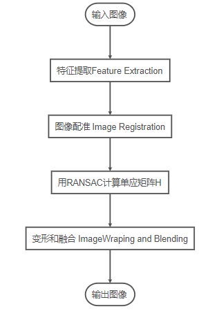
Feature Extraction: Detect feature points in all input images.Image Registration: Establish the geometric correspondence between images, allowing them to be transformed, compared, and analyzed in a common reference frame. This can be broadly categorized into several types:

Algorithms that directly use the pixel values of images, such as correlation methods.
Algorithms processed in the frequency domain, such as FFT-based methods;
Low-level feature algorithms, typically using edges and corners, such as feature-based methods.
High-level feature algorithms, typically using overlapping portions of image objects and feature relationships, such as graph-theoretic methods.

Image Warping: Image warping refers to reprojecting one image and placing it on a larger canvas.

Image Blending: Image blending is achieved by changing the grayscale levels near the boundaries of images to remove seams and create a smooth transition between images. Blend modes are used to merge two layers together.

Feature Point Extraction

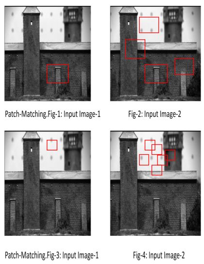
Features are elements in the two input images to be matched, which are within image patches. These patches are groups of pixels in the image. Patch matching is performed on the input images. The explanation is as follows: As shown in the figure below, fig1 and fig2 provide a good patch match because a patch in fig2 looks very similar to a patch in fig1. When considering fig3 and fig4, the patches do not match because fig4 has many similar patches that appear very similar to the patch in fig3. Due to the close proximity of pixel intensities, precise feature matching cannot be performed.

To provide better feature matching for image pairs, corner matching is used for quantitative measurement. Corners are good matching features. Corner features are stable under viewpoint changes, and the neighborhood of corners exhibits significant intensity variations. Corner detection algorithms are utilized for detecting corners in images. Corner detection algorithms include Harris corner detection, SIFT (Scale Invariant Feature Transform), FAST corner detection, and SURF (Speeded-up Robust Feature).

Harris Corner Detection Algorithm

The Harris algorithm is a point feature extraction algorithm based on the Moravec algorithm. In 1988, C. Harris and M.J Stephens designed a local detection window for images. By moving the window a small amount in different directions, the average intensity variation can be determined. We can easily identify corners by observing the intensity values within the small window. When moving the window, flat regions do not show intensity variations in all directions. Edge regions do not change intensity along the edge direction. For corners, significant intensity changes occur in all directions. The Harris corner detector provides a mathematical method for detecting flat areas, edges, and corners. The features detected by Harris are numerous, exhibiting rotation invariance and scale variance.

Under displacement:Intensity variation:where is the window function, 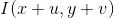is the intensity after moving, and is the intensity at a single pixel location.

The Harris corner detection algorithm is as follows:

Calculate the autocorrelation matrix for each pixel point in the image:

where is the partial derivative of .
Apply Gaussian filtering to each pixel point in the image to obtain a new matrix where the discrete two-dimensional zero-mean Gaussian function is
Calculate the corner measure for each pixel point (x,y) to obtain where ranges from .
Select local maximum points. The Harris method considers that feature points correspond to the pixel values of local maximum interest points.
Set a threshold T to detect corners. If the local maximum value of exceeds the threshold then this point is a corner.

SIFT Corner Detection Algorithm

The SIFT algorithm is a scale-invariant feature point detection algorithm that can be used to recognize similar targets in other images. The image features of SIFT are represented as key-point descriptors. When checking for image matches, two sets of key-point descriptors are provided as input to Nearest Neighbor Search (NNS), generating a tightly matched key-point descriptor (matching key-point descriptors).

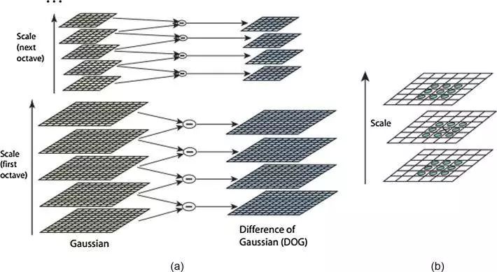The computation of SIFT is divided into four stages:

Scale-space construction.
Scale-space extrema detection.
Key-point localization.
Orientation assignment and defining key-point descriptors.

The first stage determines potential interest points. It searches all scales and image locations using the difference of Gaussian function (DOG). The locations and scales of all interest points discovered in the first stage are determined. Key points are selected based on their stability. A stable key point can resist image distortion. In the orientation assignment phase, the SIFT algorithm calculates the directions of gradients around stable key points. One or more orientations are assigned to each key point based on local image gradient directions. For a set of input frames, SIFT extracts features. Image matching uses the Best Bin First (BBF) algorithm to estimate initial matching points between input frames. To eliminate unwanted corners not belonging to the overlapping region, the RANSAC algorithm is used. It removes erroneous matches in the image pairs. The reprojection of frames is achieved by defining the size, length, and width of the frames. Finally, stitching occurs to obtain the final output stitched image. During stitching, it checks whether each pixel in each frame of the scene belongs to the distorted second frame. If so, the pixel value is assigned from the corresponding pixel in the first frame. The SIFT algorithm exhibits both rotation invariance and scale invariance. It is well-suited for target detection in high-resolution images. It is a robust image comparison algorithm, although it is slower. The running time of the SIFT algorithm is significant because comparing two images requires more time.

FAST Algorithm

FAST is a corner detection algorithm created by Trajkovic and Hedley in 1998. For FAST, corner detection outperforms edge detection because corners exhibit two-dimensional intensity changes, making them easy to distinguish from neighboring points. It is suitable for real-time image processing applications.

The FAST corner detector should meet the following requirements:

The detected locations should be consistent, insensitive to noise variations, and should not move across multiple images of the same scene.
Accuracy; the detected corners should be as close to the correct location as possible.
Speed; the corner detector should be fast enough.

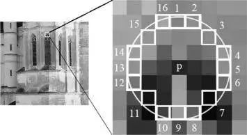
Principle: First, select 16 pixel points around a candidate corner point. If n (generally 12) of the continuous pixels are either greater than the candidate corner point plus a threshold or less than the candidate corner point minus a threshold, then this point is a corner (as shown in figure 4).

To speed up the FAST algorithm, a corner response function (CRF) is typically used. This function provides a numerical value for corner intensity based on the local neighborhood’s image intensity. The CRF is calculated for the image, and the local maxima of the CRF are taken as corners, using multi-grid techniques to enhance the algorithm’s computational speed and suppress detected false corners. FAST is an accurate and fast algorithm with good positioning (location accuracy) and high point reliability. The challenge in FAST’s corner detection algorithm lies in selecting the optimal threshold.

SURF Algorithm

Speed-up Robust Feature (SURF) corner detector employs three feature detection steps: Detection, Description, and Matching. SURF accelerates the detection process by considering the quality of detected points. It focuses more on speeding up the matching step. Using the Hessian matrix and low-dimensional descriptors significantly improves matching speed. SURF has been widely applied in the computer vision community. SURF is very effective and robust in invariant feature localization.

Image Registration

After feature points are detected, we need to associate them in some way, which can be determined using methods like NCC or SDD (Sum of Squared Differences).

Normalized Cross Correlation (NCC)

The principle of cross-correlation is to analyze the pixel windows around each point in the first image and associate them with the pixel windows around each point in the second image. The points with the highest bidirectional correlation are taken as corresponding pairs.

Calculate the similarity between the “windows” of each displacement (shifts) in the two images based on image intensity values.

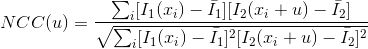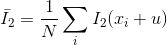
where is the average value image of the window and are the two images. is the pixel coordinates of the window, and is the displacement or offset calculated by the NCC coefficient. The range of the NCC coefficient is . The peak of the NCC corresponds to the displacement parameters representing the geometric transformation between the two images. The advantage of this method is its simple calculation, but it is particularly slow. Additionally, such algorithms require significant overlap between the source images.

Mutual Information (MI)

Mutual information measures the similarity based on the number of shared information between two images.

Two images and MI is represented in terms of entropy:

Where and are the entropies of and respectively. represents the joint entropy between the two images.

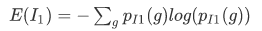
represents the possible gray values of and is the probability distribution function.

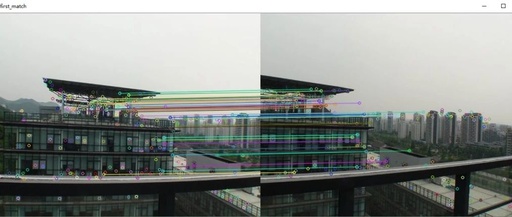
However, as we can see from the image, many points are incorrectly associated.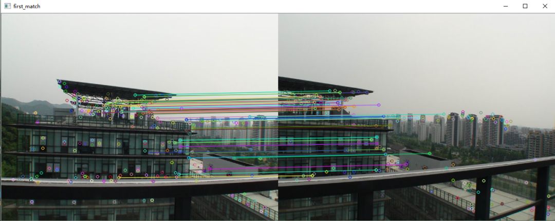

Calculating the Homography Matrix

Homography matrix estimation is the third step in image stitching. In homography matrix estimation, unwanted corners that do not belong to the overlapping area are removed. The RANSAC algorithm is used for homography.

Random Sample Consensus Algorithm (RANSAC)

The RANSAC algorithm fits a mathematical model from a dataset of observations that may contain outliers, making it an iterative method for robust parameter estimation. The algorithm is uncertain because it only produces a reasonable result with a certain probability, which increases with more iterations. The RANSAC algorithm is used to fit models robustly in the presence of a large amount of available outliers. RANSAC has many applications in computer vision.

RANSAC Principle

Randomly select a set of data from the dataset and consider it valid data (inliers) to determine the parameters of the model to be estimated. Test all data in the dataset against this model; data satisfying the model become inliers, while others are outliers (usually noise, erroneous measurements, or incorrect data points). This iteration continues until a parameter model with the maximum number of inliers is found, making it the optimal model. Consider the following assumptions:

Parameters can be estimated from N data items.
The total number of available data items is M.
The probability of randomly selected data items being part of a good model is
If a good fit exists, the probability of the algorithm exiting without finding a good fit is

RANSAC Steps

Randomly select N data (3 point pairs).
Estimate parameters x (calculate the transformation matrix H).
Based on the user-defined threshold, find the total number K of data pairs in M suitable for the model vector x (calculate the distance of each matching point after transformation to the corresponding matching point based on pre-defined thresholds, classifying matching point sets into inliers and outliers; if enough inliers exist, H is reasonable, and re-estimate H using all inliers).
If the number K of matches is sufficiently large, accept the model and exit.
Repeat steps 1-4 L times.
Exit at this step.

The value of K depends on the percentage of data we consider part of the suitable structure and how many structures exist in the image. If multiple structures exist, after a successful fit, discard the fitting data and redo RANSAC.

The number of iterations L can be calculated using the following formula:

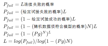
Advantages: robust estimation of model parameters. Disadvantages: no upper limit on the number of iterations, and the set number of iterations affects the algorithm’s time complexity and accuracy, requiring a predefined threshold.

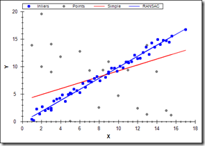
After executing RANSAC, we can only see correct matches in the image because RANSAC finds a homography matrix related to the majority of points and discards incorrect matches as outliers.

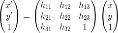
Homography

With two sets of corresponding points established, we need to establish a transformation relationship between the two sets of points, which is the image transformation relationship. Homography represents the mapping between two spaces, commonly used to represent the correspondence between two images of the same scene, allowing for matching most related feature points and achieving large area overlap through image projection.

Let the matching points of the two images be and 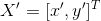, which must satisfy the formula:

and since the two vectors are collinear, is the transformation matrix of 8 parameters, indicating that four points determine an H.

Let then N point pairs provide 2N linear constraints.

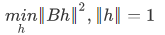
Estimate H using the RANSAC method:

First, detect corners in both images.
Apply variance-normalized correlation between corners, collecting pairs with sufficiently high correlation to form a set of candidate matches.
Select four points and calculate H.
Select pairs consistent with homography. If for certain thresholds: Dist(Hp, q) < ε, then the point pair (p, q) is considered consistent with homography H.
Repeat steps 3-4 until enough point pairs satisfy H.
Recalculate H using all qualifying point pairs through the formula.

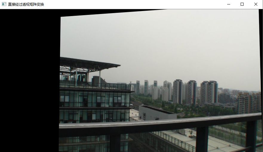
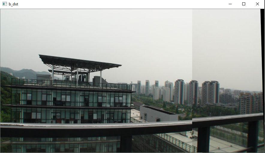
Image Warping and Blending

The final step is to warp and blend all input images into a conforming output image. Essentially, we can simply warp all input images onto a plane known as the composite panorama plane.

Image Warping Steps

First, calculate the warped image coordinate range for each input image to determine the output image size, which can be easily determined by mapping the four corners of each source image and calculating the minimum and maximum values of coordinates (x,y). Finally, calculate the offset of the specified reference image origin relative to the output panorama’s offset xoffset and offset yoffset.
The next step is to use the reverse warping described above to map the pixels of each input image onto the plane defined by the reference image, performing both forward and reverse warping of points.

Smoothing transition methods for image blending include feathering, pyramid, and gradient.

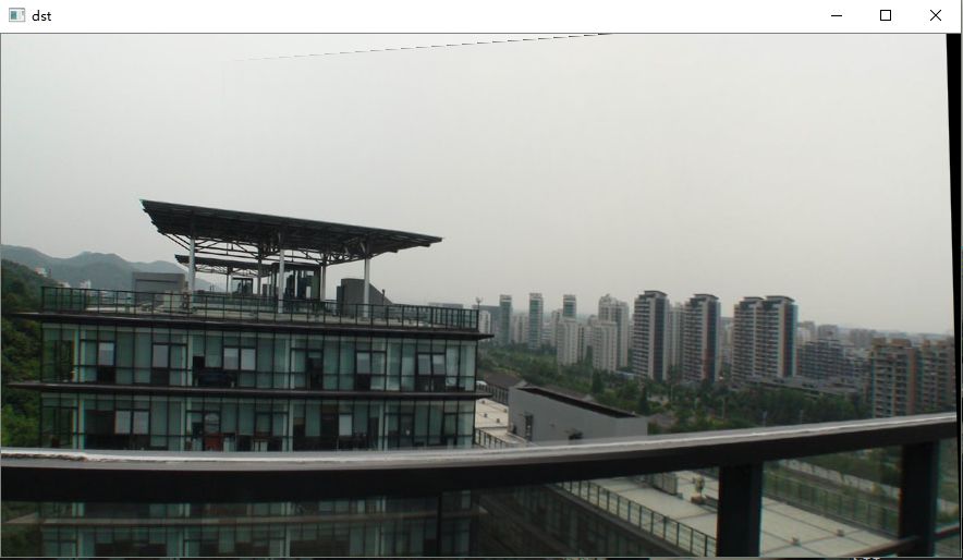
Graphical Blending

The final step is to blend pixel colors in the overlapping regions to avoid seams. The simplest available form is feathering, which uses a weighted average color value to blend overlapping pixels. Typically, we use an alpha factor, commonly referred to as the alpha channel, which has a value of 1 at the center pixel and linearly decreases to 0 at the boundary pixel. When there are at least two overlapping images in the output stitched image, we will use the following alpha values to calculate the color at one pixel: assuming two images overlap in the output image; each pixel in the image , where (R,G,B) are the color values of the pixel, we will calculate the pixel value at (x, y) in the stitched output image:

Conclusion

The above content provides a brief overview of some commonly used algorithms. The Harris corner detection method is robust and exhibits rotation invariance. However, it is sensitive to scale changes. The FAST algorithm has rotation invariance and scale invariance, with good execution time. However, its performance is poor in the presence of noise. The SIFT algorithm demonstrates rotation invariance and scale invariance, and is more effective under noisy conditions. It has very distinct features; however, it is affected by lighting changes. This algorithm performs well in execution time and lighting invariance.

References

OpenCV Exploration (Twenty-Four) Image Stitching and Blending Techniques
Debabrata Ghosh, Naima Kaabouch. A survey on image mosaicing techniques[J]. Journal of Visual Communication and Image Representation, 2016, 34. Address
Overview of Image Stitching

Academic Exchange Group

Welcome to join the WeChat group for readers to exchange with peers. Currently, there are WeChat groups for SLAM, Algorithm Competitions, Image Detection and Segmentation, Face and Body, Medical Imaging, and Comprehensive (which will gradually be subdivided) Please scan the WeChat ID below to join the group, and note: “Nickname + School/Company + Research Direction”. For example: “Zhang San + Shanghai Jiao Tong University + Visual SLAM”. Please follow the format for notes; otherwise, it will not be approved. After successful addition, invitations to relevant WeChat groups will be sent based on research direction. Please do not send advertisements in the group; otherwise, you will be removed. Thank you for your understanding~

Learn core SLAM technologies from scratch, scan to view the introduction, unconditional refund within 3 days.

Learning should not be done alone; a good learning circle can help you get started quickly, and exchanging discussions can help you avoid detours and progress quickly!

If you have needs for internships, job hunting, recruitment, project cooperation, consulting services, etc. in the AI field, come join us. We look forward to connecting with you, making it easier to find people and technology!

Introduction to Computer Vision: Image Stitching Techniques