Introduction to Attention Mechanisms in Three Transformer Models and PyTorch Implementation

We will discuss not only the theoretical concepts but also implement these attention mechanisms from scratch using Python and PyTorch. Through actual coding, we can gain a deeper understanding of the internal workings of these mechanisms.

Table of Contents

1. Self-Attention Mechanism

• Theoretical Foundations
• PyTorch Implementation
• Multi-Head Attention Extension

• Concept Introduction
• Differences from Self-Attention
• PyTorch Implementation

• Applications in Language Models
• Implementation Details
• Optimization Techniques

Through this structure, we will gradually provide a comprehensive understanding of each attention mechanism from theory to practice. Let’s start with the self-attention mechanism, which is a foundational component of the Transformer architecture.

Overview of Self-Attention

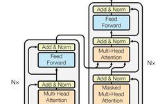
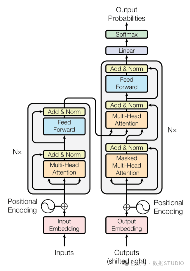
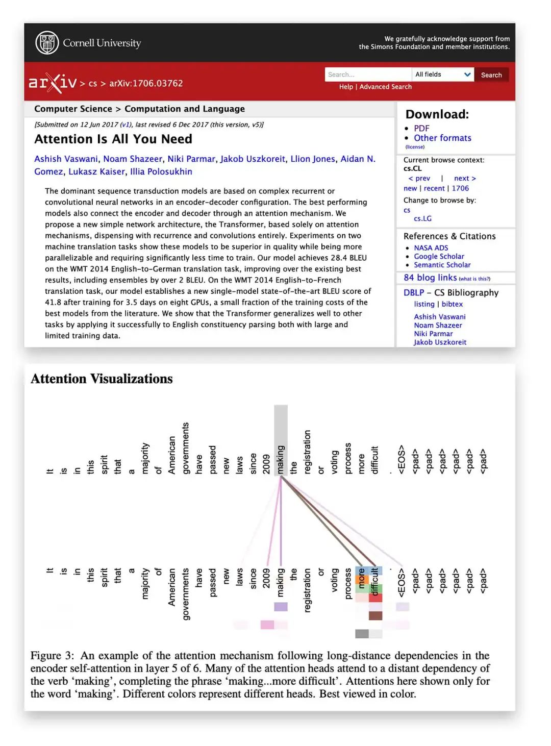
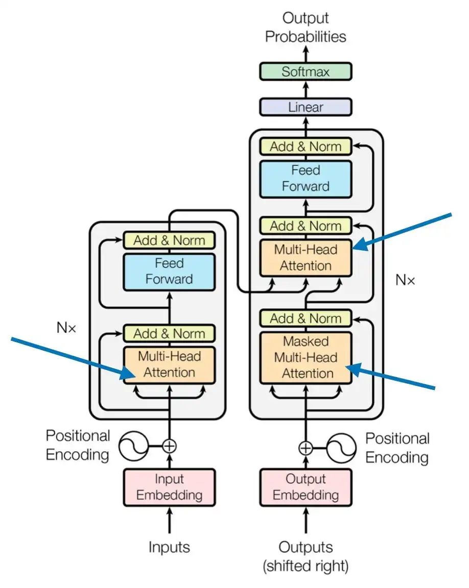
The self-attention mechanism has become central to state-of-the-art deep learning models since its introduction in the groundbreaking paper “Attention Is All You Need” in 2017, particularly in the field of natural language processing (NLP). Given its widespread application, it is crucial to understand how self-attention operates.

In deep learning, the introduction of the concept of “attention” was initially aimed at improving the ability of recurrent neural networks (RNNs) to process long sequences or sentences. For example, in machine translation tasks, word-for-word translation often fails to capture the complex grammar and expressions of a language, resulting in poor translation quality.

To address this issue, attention mechanisms allow models to consider the entire input sequence at each step, selectively focusing on the most relevant parts of the context. The Transformer architecture introduced in 2017 further developed this concept by integrating self-attention as an independent mechanism, making RNNs no longer necessary.

Self-attention allows the model to enhance the input embeddings by integrating contextual information, enabling it to dynamically weigh the importance of different elements in the sequence. This feature is especially valuable in NLP, as the meaning of words often changes depending on their context in a sentence or document.

Although many efficient versions of self-attention have been proposed, the original scaled dot-product attention mechanism introduced in “Attention Is All You Need” remains the most widely used. Due to its excellent practical performance and computational efficiency in large-scale Transformer models, it continues to serve as the foundation for many models.

Input Sentence Embedding

Before delving into the self-attention mechanism, let’s illustrate the process using an example sentence “The sun rises in the east”. Similar to other text processing models (such as recurrent or convolutional neural networks), the first step is to create sentence embeddings.

To simplify the explanation, our dictionary dc only includes the words in the input sentence. In practice, dictionaries are typically built from a larger vocabulary, generally containing 30,000 to 50,000 words.

 sentence = 'The sun rises in the east'  
 
dc = {s:i for i,s in enumerate(sorted(sentence.split()))}  
 
print(dc)

Output:

 {'The': 0, 'east': 1, 'in': 2, 'rises': 3, 'sun': 4, 'the': 5}

Next, we use this dictionary to convert each word in the sentence to its corresponding integer index.

 import torch  
 
sentence_int = torch.tensor(  
    [dc[s] for s in sentence.split()]  
)  
print(sentence_int)

Output:

 tensor([0, 4, 3, 2, 5, 1])

With this integer representation of the input sentence, we can use an embedding layer to convert each word into a vector. To simplify the demonstration, we are using a 3-dimensional embedding here, but in practice, the embedding dimensions are usually much larger (for example, 4,096 dimensions used in the Llama 2 model). Smaller dimensions help to intuitively understand the vectors without cluttering the page with numbers.

Since the sentence contains 6 words, the embedding will generate a 6×3 matrix.

 vocab_size = 50_000  
 
torch.manual_seed(123)  
embed = torch.nn.Embedding(vocab_size, 3)  
embedded_sentence = embed(sentence_int).detach()  
 
print(embedded_sentence)  
print(embedded_sentence.shape)

Output:

 tensor([[ 0.3374, -0.1778, -0.3035],  
        [ 0.1794, 1.8951, 0.4954],  
        [ 0.2692, -0.0770, -1.0205],  
        [-0.2196, -0.3792, 0.7671],  
        [-0.5880, 0.3486, 0.6603],  
        [-1.1925, 0.6984, -1.4097]])  
 torch.Size([6, 3])

This 6×3 matrix represents the embedded version of the input sentence, with each word encoded as a 3-dimensional vector. While the embedding dimensions in actual models are usually much higher, this simplified example helps us understand how embeddings work.

Weight Matrix of Scaled Dot-Product Attention

After completing the input embedding, let’s first explore the self-attention mechanism, particularly the widely used scaled dot-product attention, which is a core element of the Transformer model.

The scaled dot-product attention mechanism uses three weight matrices: Wq, Wk, and Wv. These matrices are optimized during model training and are used to transform the input data.

Transforming Queries, Keys, and Values

The weight matrices project the input data into three components:

1. Query (q)
2. Key (k)
3. Value (v)

These components are computed through matrix multiplication:

• Query: q(i) = x(i)Wq
• Key: k(i) = x(i)Wk
• Value: v(i) = x(i)Wv

Here, ‘i’ represents the position of the token in the input sequence of length T.

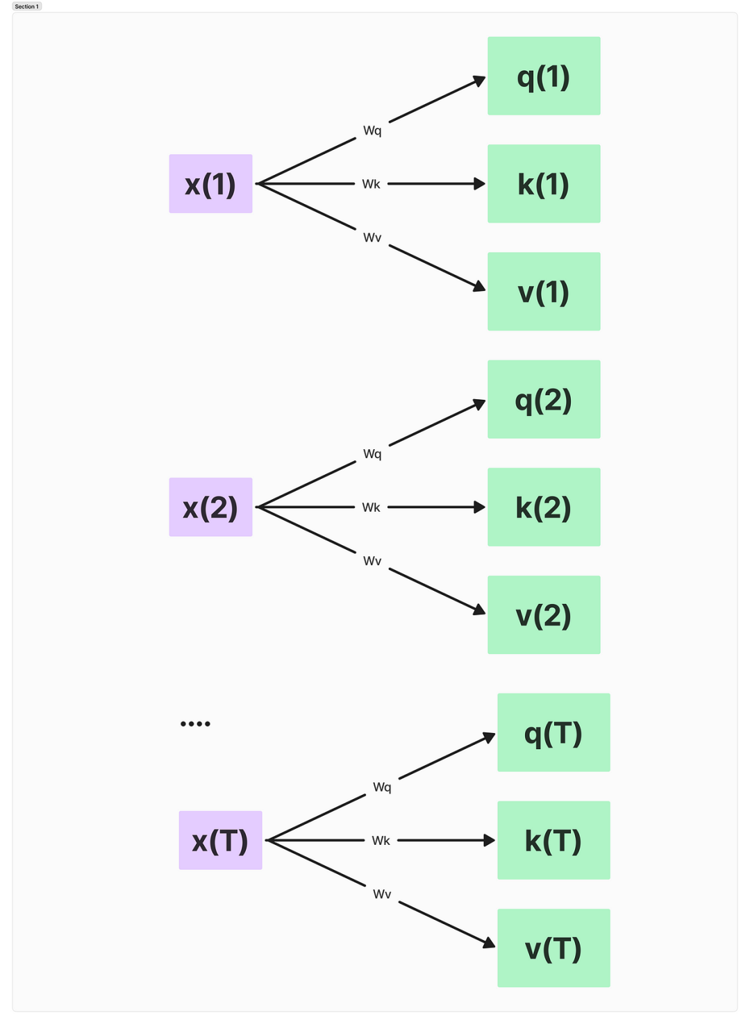
This operation effectively projects each input token x(i) into these three different spaces.

Regarding dimensions, both q(i) and k(i) are vectors with dk elements. The projection matrices Wq and Wk have shapes of d × dk, while Wv has a shape of d × dv. Here, d is the size of each word vector x.

It is important to note that q(i) and k(i) must have the same number of elements (dq = dk), as their dot product will be computed later. Many large language models simplify this by setting dq = dk = dv, but the size of v(i) can differ as needed.

Here is a code example:

 torch.manual_seed(123)  
 
d = embedded_sentence.shape[1]  
 
d_q, d_k, d_v = 2, 2, 4  
 
W_query = torch.nn.Parameter(torch.rand(d, d_q))  
W_key = torch.nn.Parameter(torch.rand(d, d_k))  
W_value = torch.nn.Parameter(torch.rand(d, d_v))

In this example, dq and dk are set to 2, while dv is set to 4. In practice, these dimensions are usually much larger, and small values are used here for conceptual clarity.

By manipulating these matrices and dimensions, we can control how the model attends to different parts of the input to capture complex relationships and dependencies in the data.

Calculating Unnormalized Attention Weights in Self-Attention Mechanism

In the self-attention mechanism, calculating the unnormalized attention weights is a key step. Below, we will demonstrate this process using the third element of the input sequence (index 2) as the query.

First, project this input element into the query, key, and value spaces:

 x_3 = embedded_sentence[2]  # Third element (index 2)
query_3 = x_3 @ W_query  
key_3 = x_3 @ W_key  
value_3 = x_3 @ W_value  
 
print("Query shape:", query_3.shape)  
print("Key shape:", key_3.shape)  
print("Value shape:", value_3.shape)

Output:

Query shape: torch.Size([2])  
Key shape: torch.Size([2])  
Value shape: torch.Size([4])

These shapes correspond to the previously set d_q = d_k = 2 and d_v = 4. Next, calculate the keys and values for all input elements:

keys = embedded_sentence @ W_key  
values = embedded_sentence @ W_value  

print("All keys shape:", keys.shape)  
print("All values shape:", values.shape)

Output:

All keys shape: torch.Size([6, 2])  
All values shape: torch.Size([6, 4])

Calculate the unnormalized attention weights. This is achieved by taking the dot product of the query with each key. For query_3:

omega_3 = query_3 @ keys.T  
print("Unnormalized attention weights for query 3:")  
print(omega_3)

Output:

Unnormalized attention weights for query 3:  
tensor([ 0.8721, -0.5302,  2.1436, -1.7589,  0.9103,  1.3245])

These six values represent the compatibility scores of our third input (the query) with each input in the sequence.

To better understand the meaning of these scores, let’s look at the highest and lowest scores:

max_score = omega_3.max()  
min_score = omega_3.min()  
max_index = omega_3.argmax()  
min_index = omega_3.argmin()  

print(f"Highest compatibility: {max_score:.4f} with input {max_index+1}")  
print(f"Lowest compatibility: {min_score:.4f} with input {min_index+1}")  

Output:

Highest compatibility: 2.1436 with input 3  
Lowest compatibility: -1.7589 with input 4

It is noteworthy that the third input (our query) has the highest compatibility with itself. This is common in self-attention since an input often contains highly relevant information related to its own context. In this example, the fourth input seems to have the lowest correlation with our query.

These unnormalized attention weights provide a raw measure of how much each input should influence the representation of our query input. They capture the initial relationships between different parts of the input sequence, laying the groundwork for the model to understand complex dependencies in the data.

In practical applications, these scores will be further processed (e.g., softmax normalization) to obtain the final attention weights, but this initial step plays a crucial role in determining the relative importance of each input element.

Normalization of Attention Weights and Context Vector Calculation

After calculating the unnormalized attention weights (ω), the next key step in the self-attention mechanism is to normalize these weights and use them to calculate the context vector. This process enables the model to focus on the most relevant parts of the input sequence.

First, we normalize the unnormalized attention weights. Using the softmax function and scaling by 1/√(dk), where dk is the dimension of the key vectors:

import torch.nn.functional as F  

d_k = 2  # Dimension of key vectors  
omega_3 = query_3 @ keys.T  # Using previous example  

attention_weights_3 = F.softmax(omega_3 / d_k**0.5, dim=0)  
print("Normalized attention weights for input 3:")  
print(attention_weights_3)

Output:

Normalized attention weights for input 3:  
tensor([0.1834, 0.0452, 0.6561, 0.0133, 0.1906, 0.2885])

The scaling (1/√dk) is crucial for maintaining appropriate gradient sizes as model depth increases, facilitating stable training. Without this scaling, the dot product could become excessively large, pushing the softmax function into regions of very small gradients.

Next, let’s explain these normalized weights:

max_weight = attention_weights_3.max()  
max_weight_index = attention_weights_3.argmax()  

print(f"Input {max_weight_index+1} has the highest attention weight: {max_weight:.4f}")

Output:

Input 3 has the highest attention weight: 0.6561

We can see that the third input (our query) received the highest attention weight, which is a common phenomenon in self-attention mechanisms.

The final step is to compute the context vector. This vector is the weighted sum of the value vectors, where the weights are our normalized attention weights:

context_vector_3 = attention_weights_3 @ values  

print("Context vector shape:", context_vector_3.shape)  
print("Context vector:")  
print(context_vector_3)

Output:

Context vector shape: torch.Size([4])  
Context vector:  
tensor([0.6237, 0.9845, 1.0523, 1.2654])

This context vector represents the original input (here x(3)) enriched by the information from all other inputs, weighted according to the relevance determined by the attention mechanism.

Our context vector has 4 dimensions, matching the previously chosen dv = 4. This dimension can be selected independently of the input dimension, providing flexibility in model design.

Thus, the original input has been transformed into a context-aware representation. This vector not only contains information from the input itself but also incorporates relevant information from the entire sequence, weighted according to the computed attention scores. This ability to dynamically focus on relevant parts of the input is a key reason why Transformer models excel in processing sequential data.

PyTorch Implementation of Self-Attention

To facilitate integration into larger neural network architectures, the self-attention mechanism can be encapsulated as a PyTorch module. Below is the implementation of the SelfAttention class, which encompasses the entire self-attention process we discussed earlier:

import torch  
import torch.nn as nn  

class SelfAttention(nn.Module):  
    def __init__(self, d_in, d_out_kq, d_out_v):  
        super().__init__()  
        self.d_out_kq = d_out_kq  
        self.W_query = nn.Parameter(torch.rand(d_in, d_out_kq))  
        self.W_key = nn.Parameter(torch.rand(d_in, d_out_kq))  
        self.W_value = nn.Parameter(torch.rand(d_in, d_out_v))  
  
    def forward(self, x):  
        keys = x @ self.W_key  
        queries = x @ self.W_query  
        values = x @ self.W_value  
          
        attn_scores = queries @ keys.T  
        attn_weights = torch.softmax(  
            attn_scores / self.d_out_kq**0.5, dim=-1  
        )  
          
        context_vec = attn_weights @ values  
        return context_vec

This class encapsulates the following steps:

1. Projecting input into key, query, and value spaces
2. Calculating attention scores
3. Scaling and normalizing attention weights
4. Generating the final context vector

Key component explanations:

• In __init__, we initialize the weight matrices as nn.Parameter objects, allowing PyTorch to automatically track and update them during training.
• The forward method succinctly implements the entire self-attention process.
• We use the @ operator for matrix multiplication, which is equivalent to torch.matmul.
• The scaling factor self.d_out_kq**0.5 is applied before softmax, as discussed.

Using this SelfAttention module is demonstrated below:

torch.manual_seed(123)  
  
d_in, d_out_kq, d_out_v = 3, 2, 4  
  
sa = SelfAttention(d_in, d_out_kq, d_out_v)  
  
# Assume embedded_sentence is our input tensor  
output = sa(embedded_sentence)  
print(output)

Output:

tensor([[-0.1564,  0.1028, -0.0763, -0.0764],  
        [ 0.5313,  1.3607,  0.7891,  1.3110],  
        [-0.3542, -0.1234, -0.2627, -0.3706],  
        [ 0.0071,  0.3345,  0.0969,  0.1998],  
        [ 0.1008,  0.4780,  0.2021,  0.3674],  
        [-0.5296, -0.2799, -0.4107, -0.6006]], grad_fn=<MmBackward0>)

Each row in this output tensor represents the context vector for the corresponding input token. Notably, the second row [0.5313, 1.3607, 0.7891, 1.3110] matches the result we previously calculated for the second input element.

This implementation is efficient and can process all input tokens in parallel. It also provides flexibility, allowing us to easily change the dimensions of key/query and value projections by adjusting d_out_kq and d_out_v parameters.

Multi-Head Attention Mechanism: An Advanced Extension of Self-Attention

The multi-head attention mechanism is a powerful extension of the self-attention mechanism discussed earlier. It allows the model to simultaneously focus on information from different representation subspaces at different positions. Below, we will analyze this concept in detail and implement it.

Core Concept of Multi-Head Attention

The main features of the multi-head attention mechanism include:

1. Creating multiple sets of query, key, and value weight matrices.
2. Each set of matrices forms an “attention head”.
3. Each head can focus on different aspects of the input sequence.
4. All heads’ outputs are concatenated and linearly transformed to generate the final output.

This approach enables the model to capture various types of relationships and patterns in the data simultaneously.

Implementation of Multi-Head Attention

Below is the implementation of the MultiHeadAttentionWrapper class, which utilizes our previously defined SelfAttention class:

class MultiHeadAttentionWrapper(nn.Module):  
    def __init__(self, d_in, d_out_kq, d_out_v, num_heads):  
        super().__init__()  
        self.heads = nn.ModuleList(  
            [SelfAttention(d_in, d_out_kq, d_out_v)   
             for _ in range(num_heads)]  
        )  
  
    def forward(self, x):  
        return torch.cat([head(x) for head in self.heads], dim=-1)

Using this multi-head attention wrapper:

torch.manual_seed(123)  
  
d_in, d_out_kq, d_out_v = 3, 2, 1  
num_heads = 4  
  
mha = MultiHeadAttentionWrapper(d_in, d_out_kq, d_out_v, num_heads)  
  
context_vecs = mha(embedded_sentence)  
  
print(context_vecs)  
print("context_vecs.shape:", context_vecs.shape)

Output:

tensor([[-0.0185,  0.0170,  0.1999, -0.0860],  
        [ 0.4003,  1.7137,  1.3981,  1.0497],  
        [-0.1103, -0.1609,  0.0079, -0.2416],  
        [ 0.0668,  0.3534,  0.2322,  0.1008],  
        [ 0.1180,  0.6949,  0.3157,  0.2807],  
        [-0.1827, -0.2060, -0.2393, -0.3167]], grad_fn=<CatBackward0>)  
context_vecs.shape: torch.Size([6, 4])

Advantages of Multi-Head Attention

1. Diverse Feature Learning: Each head can learn to focus on different aspects of the input. For example, one head might focus on local relationships while another captures long-range dependencies.
2. Enhanced Model Capacity: Multiple heads allow the model to represent more complex relationships in the data without significantly increasing the number of parameters.
3. Parallel Processing Efficiency: The independence of each head allows for efficient parallel computation on GPUs or TPUs.
4. Improved Model Stability and Robustness: Using multiple heads can make the model more robust, as it is less likely to overfit to specific patterns captured by a single attention mechanism.

Comparison of Multi-Head Attention with Single Head Large Output

While increasing the output dimension of a single self-attention head (for example, setting d_out_v = 4 in a single head) may seem similar to using multiple heads, there are key differences:

1. Independent Learning Capability: Each head in multi-head attention learns its own set of query, key, and value projections, allowing for more diverse feature extraction.
2. Computational Efficiency Advantage: Multi-head attention can be parallelized more efficiently, potentially leading to faster training and inference speeds.
3. Ensemble Learning Effect: The roles of multiple heads are similar to an ensemble of attention mechanisms, where each head may specialize in different aspects of the input.

Practical Application Considerations

In practical applications, the number of attention heads is an adjustable hyperparameter. For example, the 7B parameter Llama 2 model uses 32 attention heads. The choice of the number of heads typically depends on the specific task, model size, and available computational resources.

By leveraging the multi-head attention mechanism, Transformer models can capture a rich set of relationships in the input data, which is a key factor in their outstanding performance across various natural language processing tasks.

Cross-Attention: A Bridge Connecting Different Input Sequences

Cross-attention is a powerful variant of the attention mechanism that allows the model to process information from two different input sequences. This is particularly useful in scenarios where one sequence provides information or guidance for processing the other sequence. We will now delve into the concept and implementation of cross-attention.

Core Concept of Cross-Attention

The main features of cross-attention include:

1. Processing two different input sequences.
2. Queries are generated from one sequence, while keys and values come from the other sequence.
3. Allows the model to selectively focus on parts of one sequence based on the content of another sequence.

Implementation of Cross-Attention

Below is the implementation of the CrossAttention class:

class CrossAttention(nn.Module):  
    def __init__(self, d_in, d_out_kq, d_out_v):  
        super().__init__()  
        self.d_out_kq = d_out_kq  
        self.W_query = nn.Parameter(torch.rand(d_in, d_out_kq))  
        self.W_key = nn.Parameter(torch.rand(d_in, d_out_kq))  
        self.W_value = nn.Parameter(torch.rand(d_in, d_out_v))  
  
    def forward(self, x_1, x_2):  
        queries_1 = x_1 @ self.W_query  
        keys_2 = x_2 @ self.W_key  
        values_2 = x_2 @ self.W_value  
          
        attn_scores = queries_1 @ keys_2.T  
        attn_weights = torch.softmax(  
            attn_scores / self.d_out_kq**0.5, dim=-1)  
          
        context_vec = attn_weights @ values_2  
        return context_vec

Using this cross-attention module:

torch.manual_seed(123)  
  
d_in, d_out_kq, d_out_v = 3, 2, 4  
  
crossattn = CrossAttention(d_in, d_out_kq, d_out_v)  
  
first_input = embedded_sentence  
second_input = torch.rand(8, d_in)  
  
print("First input shape:", first_input.shape)  
print("Second input shape:", second_input.shape)  
  
context_vectors = crossattn(first_input, second_input)  
  
print(context_vectors)  
print("Output shape:", context_vectors.shape)

Output:

First input shape: torch.Size([6, 3])  
Second input shape: torch.Size([8, 3])  
tensor([[0.4231, 0.8665, 0.6503, 1.0042],  
        [0.4874, 0.9718, 0.7359, 1.1353],  
        [0.4054, 0.8359, 0.6258, 0.9667],  
        [0.4357, 0.8886, 0.6678, 1.0311],  
        [0.4429, 0.9006, 0.6775, 1.0460],  
        [0.3860, 0.8021, 0.5985, 0.9250]], grad_fn=<MmBackward0>)  
Output shape: torch.Size([6, 4])

Key Differences Between Cross-Attention and Self-Attention

1. Dual Input Sequences: Cross-attention accepts two inputs, x_1 and x_2, rather than a single input.
2. Query-Key Interaction Mode: Queries come from x_1, while keys and values come from x_2.
3. Flexibility in Sequence Lengths: The two input sequences can have different lengths.

Applications of Cross-Attention

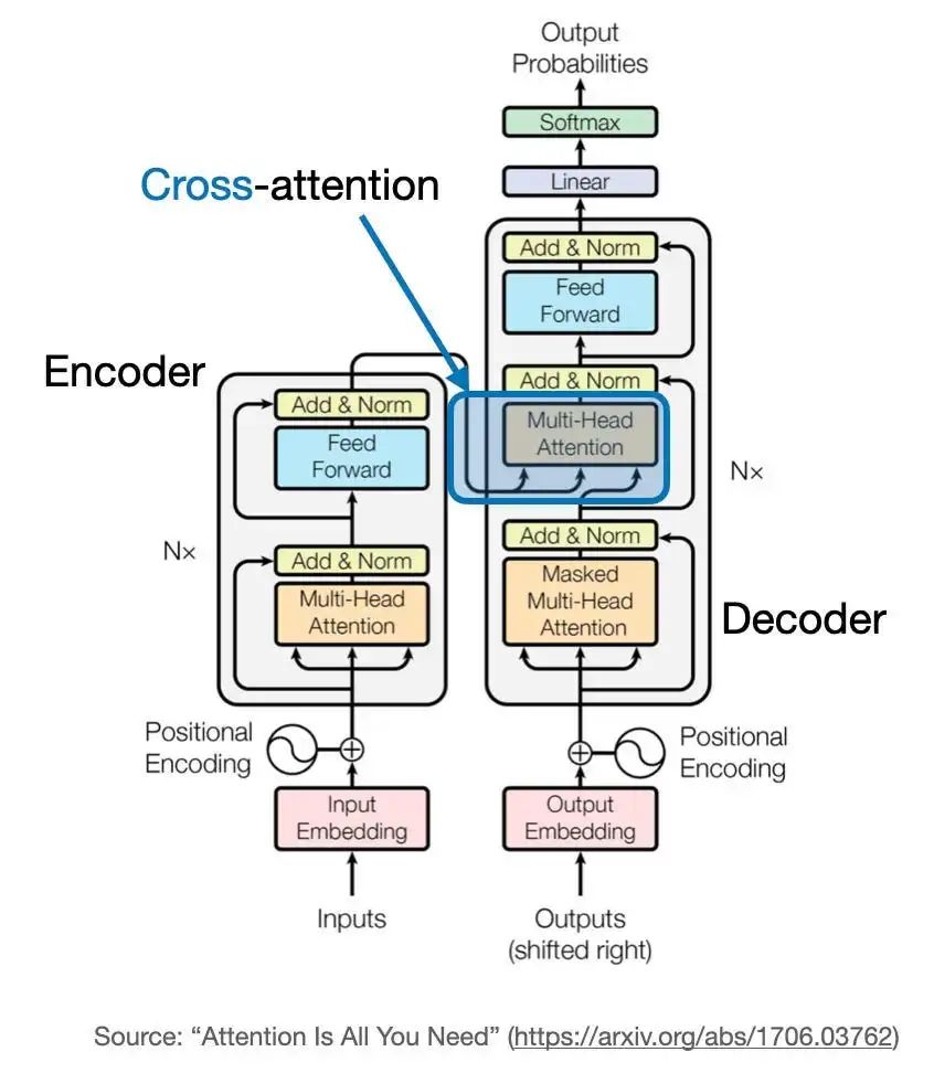
1. Machine Translation: In the original Transformer model, cross-attention allows the decoder to focus on relevant parts of the source sentence when generating translations.
2. Image Caption Generation: The model can focus on different parts of the image (represented as a sequence of image features) when generating each word of the description.
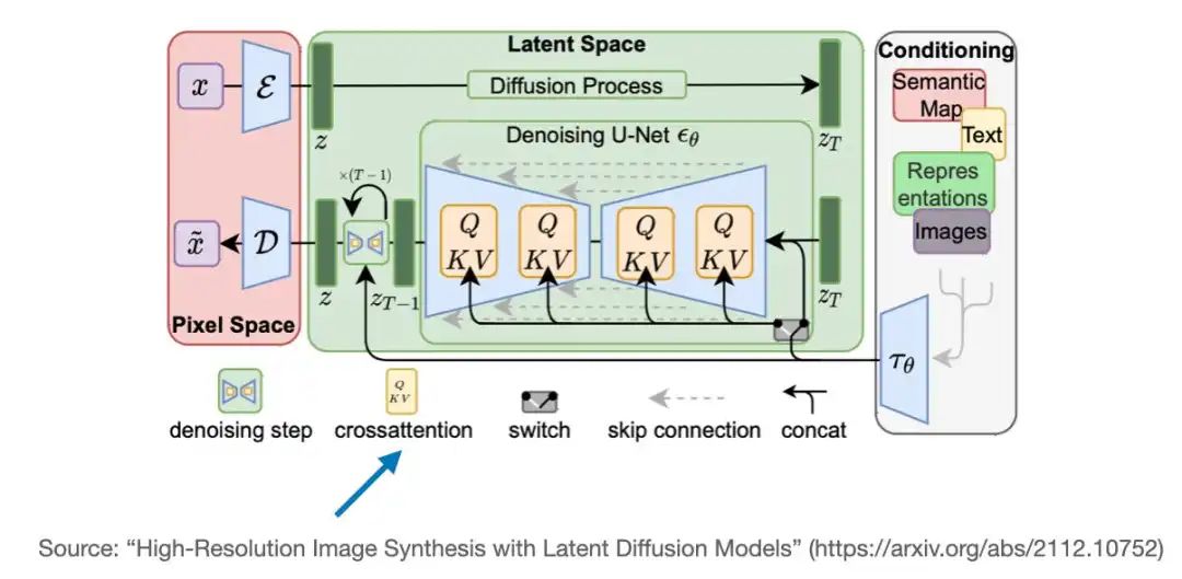
3. Stable Diffusion Model: Cross-attention is used to associate image generation with text prompts, allowing the model to integrate textual information into the visual generation process.
4. Question Answering Systems: The model can focus on different parts of the context paragraph based on the content of the question.

Advantages of Cross-Attention

1. Information Integration Capability: Allows the model to selectively integrate information from one sequence into the processing of another sequence.
2. Flexibility in Handling Multi-Modal Inputs: Can process inputs of different lengths and modalities.
3. Enhanced Interpretability: Attention weights can provide insights into how the model associates different parts of the two sequences.

Considerations in Practical Applications

• The embedding dimension (d_in) must remain consistent across both input sequences, even if they differ in length.
• For long sequences, cross-attention may be computationally intensive, requiring consideration of computational efficiency.
• Similar to self-attention, cross-attention can also be extended to multi-head versions for greater expressive power.

Cross-attention is a versatile tool that enables models to process information from multiple sources or modalities, which is crucial in many advanced AI applications. It allows for dynamic attention to relevant information between different inputs, significantly contributing to the success of models in tasks that require the integration of diverse information sources.

The Stable Diffusion model also utilizes the cross-attention mechanism. In this model, cross-attention occurs between the image features generated within the U-Net architecture and the text prompts used for guidance. This technique was initially proposed in the paper “High-Resolution Image Synthesis with Latent Diffusion Models” that introduced the concept of Stable Diffusion. Subsequently, Stability AI adopted this approach to implement the widely popular Stable Diffusion model.

Causal Self-Attention

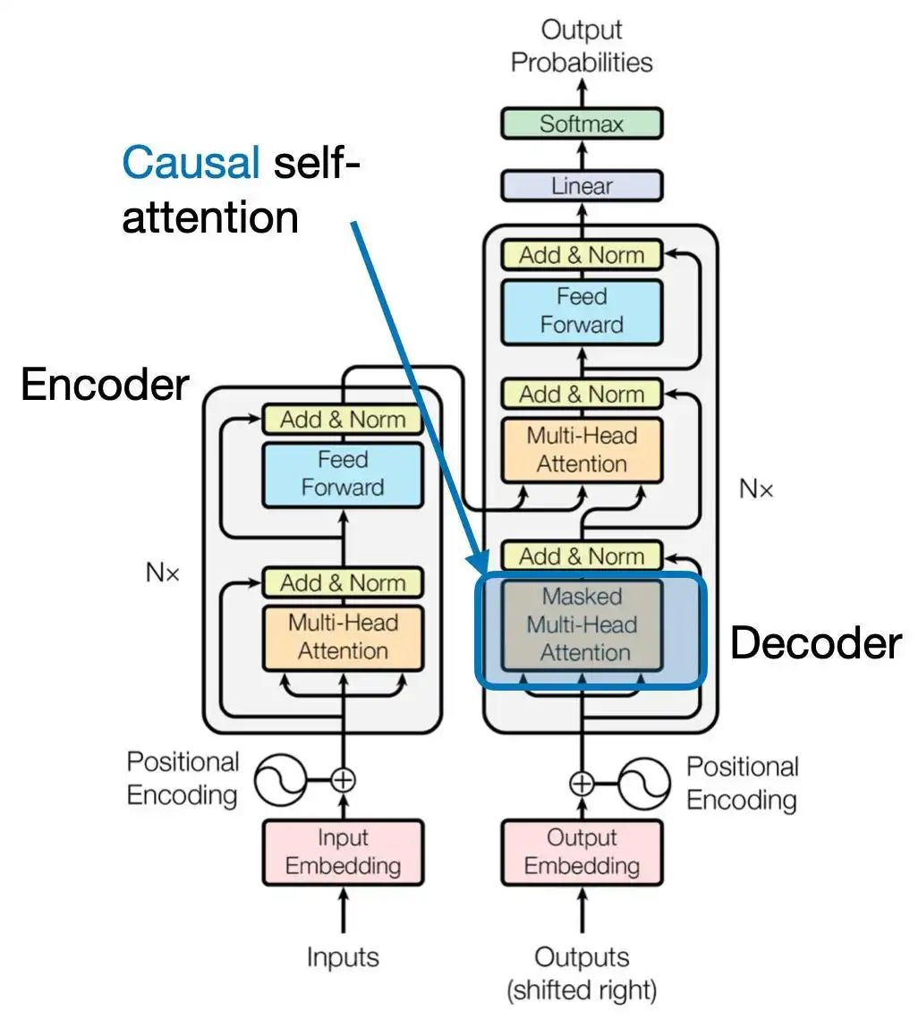
We will now introduce how to adjust the previously discussed self-attention mechanism to the causal self-attention mechanism, which is particularly suitable for text generation in GPT-style (decoder-style) large language models (LLMs). This mechanism is also known as “masked self-attention”. In the original Transformer architecture, it corresponds to the “masked multi-head attention” module. To simplify the explanation, we will focus on a single attention head, but this concept also applies to multi-head attention.

Causal self-attention ensures that the output at a given position depends only on the known outputs from previous positions in the sequence, without relying on information from subsequent positions. In short, when predicting each next word, the model should only consider the words that came before it. To implement this in GPT-style LLMs, we mask future tokens for each token being processed in the input text.

To illustrate this process, let’s consider a training text sample: “The cat sits on the mat”. In causal self-attention, we would have the following setup, where the context vector for the words on the right side of the arrow should only contain itself and the preceding words:

“The” → “cat”
“The cat” → “sits”
“The cat sits” → “on”
“The cat sits on” → “the”
“The cat sits on the” → “mat”

This setup ensures that when generating text, the model only uses the information available at each step of the generation process.

Referring back to the attention score calculation from the self-attention section:

torch.manual_seed(123)  
  
d_in, d_out_kq, d_out_v = 3, 2, 4  
  
W_query = nn.Parameter(torch.rand(d_in, d_out_kq))  
W_key = nn.Parameter(torch.rand(d_in, d_out_kq))  
W_value = nn.Parameter(torch.rand(d_in, d_out_v))  
  
x = embedded_sentence  
  
keys = x @ W_key  
queries = x @ W_query  
values = x @ W_value  
  
attn_scores = queries @ keys.T   
  
print(attn_scores)  
print(attn_scores.shape)

Output:

tensor([[ 0.0613, -0.3491,  0.1443, -0.0437, -0.1303,  0.1076],  
        [-0.6004,  3.4707, -1.5023,  0.4991,  1.2903, -1.3374],  
        [ 0.2432, -1.3934,  0.5869, -0.1851, -0.5191,  0.4730],  
        [-0.0794,  0.4487, -0.1807,  0.0518,  0.1677, -0.1197],  
        [-0.1510,  0.8626, -0.3597,  0.1112,  0.3216, -0.2787],  
        [ 0.4344, -2.5037,  1.0740, -0.3509, -0.9315,  0.9265]],  
       grad_fn=<MmBackward0>)  
torch.Size([6, 6])

We obtain a 6×6 tensor representing the pairwise unnormalized attention weights (attention scores) of the 6 input tokens.

Next, we calculate the scaled dot-product attention using the softmax function:

attn_weights = torch.softmax(attn_scores / d_out_kq**0.5, dim=1)  
print(attn_weights)

Output:

tensor([[0.1772, 0.1326, 0.1879, 0.1645, 0.1547, 0.1831],  
        [0.0386, 0.6870, 0.0204, 0.0840, 0.1470, 0.0229],  
        [0.1965, 0.0618, 0.2506, 0.1452, 0.1146, 0.2312],  
        [0.1505, 0.2187, 0.1401, 0.1651, 0.1793, 0.1463],  
        [0.1347, 0.2758, 0.1162, 0.1621, 0.1881, 0.1231],  
        [0.1973, 0.0247, 0.3102, 0.1132, 0.0751, 0.2794]],  
       grad_fn=<SoftmaxBackward0>)

To implement causal self-attention, we need to mask all future tokens. The most straightforward way to do this is to apply a mask above the diagonal of the attention weight matrix. We can use PyTorch’s tril function to achieve this:

block_size = attn_scores.shape[0]  
mask_simple = torch.tril(torch.ones(block_size, block_size))  
print(mask_simple)

Output:

tensor([[1., 0., 0., 0., 0., 0.],  
        [1., 1., 0., 0., 0., 0.],  
        [1., 1., 1., 0., 0., 0.],  
        [1., 1., 1., 1., 0., 0.],  
        [1., 1., 1., 1., 1., 0.],  
        [1., 1., 1., 1., 1., 1.]])

Now, multiply the attention weights by this mask to set all attention weights above the diagonal to zero:

masked_simple = attn_weights * mask_simple  
print(masked_simple)

Output:

tensor([[0.1772, 0.0000, 0.0000, 0.0000, 0.0000, 0.0000],  
        [0.0386, 0.6870, 0.0000, 0.0000, 0.0000, 0.0000],  
        [0.1965, 0.0618, 0.2506, 0.0000, 0.0000, 0.0000],  
        [0.1505, 0.2187, 0.1401, 0.2449, 0.0000, 0.0000],  
        [0.1536, 0.3145, 0.1325, 0.1849, 0.2145, 0.0000],  
        [0.1973, 0.0247, 0.3102, 0.1132, 0.0751, 0.2794]],  
       grad_fn=<MulBackward0>)

However, this method results in the sum of attention weights in each row no longer equaling 1. To resolve this, we also need to normalize the rows:

row_sums = masked_simple.sum(dim=1, keepdim=True)  
masked_simple_norm = masked_simple / row_sums  
print(masked_simple_norm)

Output:

tensor([[1.0000, 0.0000, 0.0000, 0.0000, 0.0000, 0.0000],  
        [0.0532, 0.9468, 0.0000, 0.0000, 0.0000, 0.0000],  
        [0.3862, 0.1214, 0.4924, 0.0000, 0.0000, 0.0000],  
        [0.2232, 0.3242, 0.2078, 0.2449, 0.0000, 0.0000],  
        [0.1536, 0.3145, 0.1325, 0.1849, 0.2145, 0.0000],  
        [0.1973, 0.0247, 0.3102, 0.1132, 0.0751, 0.2794]],  
       grad_fn=<DivBackward0>)

Now, the sum of attention weights in each row equals 1, conforming to standard normalization for attention weights.

A more efficient way to achieve the same result is to mask the attention scores before applying softmax, rather than masking the attention weights afterward:

mask = torch.triu(torch.ones(block_size, block_size), diagonal=1)  
masked = attn_scores.masked_fill(mask.bool(), float('-inf'))  
print(masked)

Output:

tensor([[ 0.0613,    -inf,    -inf,    -inf,    -inf,    -inf],  
        [-0.6004,  3.4707,    -inf,    -inf,    -inf,    -inf],  
        [ 0.2432, -1.3934,  0.5869,    -inf,    -inf,    -inf],  
        [-0.0794,  0.4487, -0.1807,  0.0518,    -inf,    -inf],  
        [-0.1510,  0.8626, -0.3597,  0.1112,  0.3216,    -inf],  
        [ 0.4344, -2.5037,  1.0740, -0.3509, -0.9315,  0.9265]],  
       grad_fn=<MaskedFillBackward0>)

Now apply softmax to obtain the final attention weights:

attn_weights = torch.softmax(masked / d_out_kq**0.5, dim=1)  
print(attn_weights)

Output:

tensor([[1.0000, 0.0000, 0.0000, 0.0000, 0.0000, 0.0000],  
        [0.0532, 0.9468, 0.0000, 0.0000, 0.0000, 0.0000],  
        [0.3862, 0.1214, 0.4924, 0.0000, 0.0000, 0.0000],  
        [0.2232, 0.3242, 0.2078, 0.2449, 0.0000, 0.0000],  
        [0.1536, 0.3145, 0.1325, 0.1849, 0.2145, 0.0000],  
        [0.1973, 0.0247, 0.3102, 0.1132, 0.0751, 0.2794]],  
       grad_fn=<SoftmaxBackward0>)

This method is more efficient as it avoids unnecessary computations for masked positions and does not require re-normalization. The softmax function effectively treats -inf values as zero probability since e^(-inf) approaches 0.

Implementing causal self-attention in this way ensures that language models can generate text in a left-to-right manner, considering only previous context when predicting each new token. This is crucial for producing coherent and contextually appropriate sequences in text generation tasks.

Conclusion

In this article, we explored the inner workings of the self-attention mechanism in depth, using actual coding to understand its implementation. Building on this, we studied multi-head attention, which is a core component of large language Transformer models.

We also expanded our discussion to explore cross-attention (a variant of self-attention), particularly useful for information exchange between two different sequences. This mechanism is especially useful in tasks like machine translation or image captioning, where information from one domain needs to guide the processing of another.

Finally, we delved into causal self-attention, a key concept for generating coherent and contextually appropriate sequences in decoder-style LLMs (like GPT and Llama). This mechanism ensures that the model’s predictions are based only on previous tokens, mimicking the left-to-right nature of natural language generation.

Finally: The code presented in this article is primarily for illustrative purposes. In actual training of LLMs, the implementation of self-attention typically uses optimized versions. Techniques like Flash Attention significantly reduce memory usage and computational load, making the training of large models more efficient.