Author: fengbingchun
Original: http://blog.csdn.net/fengbingchun/article/details/50274471
1. Concept of Artificial Neural Networks
Artificial Neural Networks (ANN), abbreviated as neural networks (NN), are mathematical models that simulate the processing mechanisms of the human brain’s neural system for complex information. This model is characterized by parallel distributed processing capabilities, high fault tolerance, intelligence, and self-learning abilities. It combines information processing and storage, attracting attention from various disciplines due to its unique knowledge representation and intelligent adaptive learning capabilities. Essentially, it is a complex network composed of numerous simple interconnected components, exhibiting high non-linearity and capable of performing complex logical operations and non-linear relationship realizations.
Neural networks are computational models consisting of numerous connected nodes (or neurons). Each node represents a specific output function known as an activation function. The connection between any two nodes represents a weighted value for the signal passing through that connection, referred to as weight. Neural networks simulate human memory through this method. The output of the network depends on its structure, connection method, weights, and activation functions. The network itself typically approximates some algorithms or functions from nature, and may also express a logical strategy. The construction concept of neural networks is inspired by the operation of biological neural networks. Artificial neural networks combine the understanding of biological neural networks with mathematical statistical models, utilizing mathematical statistical tools for implementation. On the other hand, in the field of artificial perception within artificial intelligence, we enable neural networks to possess decision-making capabilities and simple judgment abilities similar to humans through mathematical statistical methods, further extending traditional logical reasoning.
In artificial neural networks, neuron processing units can represent different objects, such as features, letters, concepts, or meaningful abstract patterns. The types of processing units in the network are divided into three categories: input units, output units, and hidden units. Input units receive signals and data from the external world; output units output the results of system processing; hidden units exist between input and output units and cannot be observed from the outside. The connection weights between neurons reflect the strength of connections between units, and the representation and processing of information are reflected in the connection relationships of network processing units. Artificial neural networks are a non-programmatic, adaptive, brain-style information processing system, essentially achieving a parallel distributed information processing function through network transformations and dynamic behaviors, mimicking the information processing functions of the human brain’s neural system at varying degrees and levels.
Neural networks are a mathematical model that processes information similarly to the synaptic connection structure of brain neurons. It is simulated based on human understanding of their brain’s organization and thinking mechanisms, rooted in neurobiology, mathematics, cognitive science, artificial intelligence, statistics, physics, computer science, and engineering.
2. Development of Artificial Neural Networks
The development of neural networks has a long history. The process can be summarized in the following four stages.
1. First Stage – Enlightenment Period
(1) M-P Neural Network Model: Research on neural networks began in the 1940s.
(2) Hebb’s Rule: In 1949, psychologist Hebb published “The Organization of Behavior,” proposing the hypothesis that the strength of synaptic connections can vary.
(3) Perceptron Model: In 1957, Rosenblatt proposed the Perceptron model based on the M-P model.
(4) ADALINE Network Model: In 1959, American engineers Widrow and Hoff proposed the Adaptive Linear Element (Adaline) and the Widrow-Hoff learning rule (also known as the least mean square algorithm or δ-rule) for training neural networks.
2. Second Stage – Low Tide Period
One of the founders of artificial intelligence, Minsky, and Papert conducted an in-depth mathematical study on the functions and limitations of network systems represented by perceptrons, publishing the sensational book “Perceptrons” in 1969.
(1) Self-Organizing Neural Network SOM Model: In 1972, Professor Kohonen from Finland proposed the Self-Organizing Feature Map (SOM).
(2) Adaptive Resonance Theory ART: In 1976, American Professor Grossberg proposed the well-known Adaptive Resonance Theory (ART), which features self-organization and self-stabilization during its learning process.
3. Third Stage – Renaissance Period
(1) Hopfield Model: In 1982, American physicist Hopfield proposed a discrete neural network, the discrete Hopfield network, significantly advancing neural network research. It was the first to introduce the Lyapunov function into the network, with later researchers referring to it as the energy function, proving the network’s stability.
(2) Boltzmann Machine Model: In 1983, Kirkpatrick and others recognized that simulated annealing algorithms could solve NP-complete combinatorial optimization problems, a method that simulates the annealing process of high-temperature objects to find global optimal solutions, originally proposed by Metropolis et al. in 1953.
(3) BP Neural Network Model: In 1986, Rumelhart and others proposed the Back-Propagation (BP) algorithm for correcting weights in multilayer neural networks based on the multilayer neural network model.
(4) Parallel Distributed Processing Theory: In 1986, Rumelhart and McClelland edited “Parallel Distributed Processing: Exploration in the Microstructures of Cognition,” establishing the theory of parallel distributed processing.
(5) Cellular Neural Network Model: In 1988, Chua and Yang proposed the Cellular Neural Network (CNN) model, which is a large-scale nonlinear computational simulation system with cellular automata characteristics.
(6) Darwinism Model: The Darwinism model proposed by Edelman had a significant impact in the early 1990s, establishing a theoretical framework for neural network systems.
(7) In 1988, Linsker proposed a new self-organizing theory for perceptron networks, forming the maximum mutual information theory based on Shannon’s information theory, igniting the theory of information applications based on neural networks.
(8) In 1988, Broomhead and Lowe proposed a hierarchical network design method using Radial Basis Function (RBF), linking the design of neural networks with numerical analysis and linear adaptive filtering.
(9) In 1991, Haken introduced synergetics into neural networks, asserting that cognitive processes are spontaneous and that pattern recognition processes are pattern formation processes.
(10) In 1994, Liao Xiaoxin proposed a mathematical theory and foundation for cellular neural networks, bringing new progress to the field. By broadening the class of activation functions of neural networks, more general time-delay cellular neural networks (DCNN), Hopfield neural networks (HNN), and bidirectional associative memory networks (BAM) models were presented.
(11) In the early 1990s, Vapnik and others proposed the concepts of Support Vector Machines (SVM) and VC (Vapnik-Chervonenkis) dimensions.
After years of development, hundreds of neural network models have been proposed.
4. Fourth Stage – Peak Period [Note: This classification is self-made and may not be accurate ^_^]
Deep Learning (DL) was proposed by Hinton et al. in 2006, representing a new field of Machine Learning (ML). Deep learning essentially constructs machine learning architecture models with multiple hidden layers, training them with large-scale data to obtain a wealth of more representative feature information. Deep learning algorithms break the traditional neural network’s limitation on the number of layers, allowing designers to select the number of network layers as needed.
For articles on deep learning, please refer to: http://blog.csdn.net/fengbingchun/article/details/50087005
3. Characteristics of Artificial Neural Networks
Neural networks are an information response network topology structure composed of numerous neurons stored within the network, employing a parallel distributed signal processing mechanism, thus possessing fast processing speeds and strong fault tolerance.
1. The neural network model is used to simulate the activity process of human brain neurons, including information processing, storage, and search processes. Artificial neural networks have the following basic characteristics:
(1) High Parallelism: Artificial neural networks consist of many identical simple processing units connected in parallel. Although each neuron functions simply, the parallel processing capability and effectiveness of numerous simple neurons are quite remarkable.
(2) High Nonlinear Global Effects: Each neuron in artificial neural networks receives inputs from many other neurons and generates outputs through the parallel network, influencing other neurons. This mutual constraint and influence between networks realize the nonlinear mapping from input state to output state space. From a global perspective, the overall performance of the network is not merely the sum of local performances but exhibits some collective behavior.
(3) Associative Memory Function and Good Fault Tolerance: Artificial neural networks store processed data information in the weights between neurons through their unique network structure, possessing associative memory functionality. The information stored in a single weight cannot be discerned, resulting in a distributed storage form, which provides the network with good fault tolerance and enables tasks such as feature extraction, defect pattern restoration, clustering analysis, as well as pattern association, classification, and recognition. It can learn and make decisions from imperfect data and patterns.
(4) Good Adaptive and Self-Learning Capabilities: Artificial neural networks acquire weights and structures through learning training, presenting strong self-learning abilities and adaptability to the environment.
(5) Distributed Knowledge Storage: In neural networks, knowledge is not stored in specific storage units but is distributed throughout the system, requiring many connections to store multiple pieces of knowledge.
(6) Non-Convexity: The evolution direction of a system, under certain conditions, will depend on a specific state function. For example, the energy function, where its extreme values correspond to relatively stable states of the system. Non-convexity refers to the existence of multiple extreme values, leading to multiple stable equilibrium states of the system, which will result in the diversity of system evolution.
2. Artificial neural networks aim to mimic the structure and functions of the human brain. Therefore, they possess certain intelligent characteristics in functionality:
(1) Associative Memory Function: Due to the distributed storage of information and parallel computing capabilities, neural networks have the ability to perform associative memory for external stimuli and input information.
(2) Classification and Recognition Functions:: Neural networks have strong recognition and classification capabilities for external input samples. Classification of input samples essentially involves finding the partitioning regions that meet classification requirements in the sample space, with each region containing samples of one class.
(3) Optimization Computation Function: Optimization computation refers to finding a parameter combination under known constraints that minimizes a defined objective function.
(4) Nonlinear Mapping Function: In many practical problems, such as process control, system identification, fault diagnosis, and robot control, there exist complex nonlinear relationships between the system’s inputs and outputs, making it difficult to establish their mathematical models using traditional mathematical equations.
4. Structure of Artificial Neural Networks
1. Structure of Biological Neurons: Nerve cells are the basic units that constitute the nervous system, referred to as biological neurons, or simply neurons. Neurons mainly consist of three parts: (1) cell body; (2) axon; (3) dendrites. As shown in the figure below:
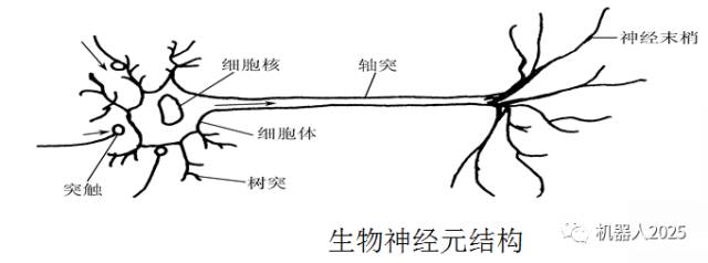
The synapse is the interface part connecting neurons, specifically the junction where the nerve endings of one neuron contact the dendrites of another, located at the end of the neuron’s nerve terminal. The brain can be viewed as a neural network composed of over 100 billion neurons. The information transmission and processing of neurons is an electrochemical activity. Dendrites receive external stimuli through electrochemical actions, reflected as axonal potentials within the cell body. When the axonal potential reaches a certain value, it generates a neural pulse or action potential, which is then transmitted to other neurons through the axonal terminals.
From the perspective of control theory, this process can be viewed as a dynamic process of a multi-input single-output nonlinear system.
Functional characteristics of neurons: (1) spatiotemporal integration function; (2) dynamic polarization of neurons; (3) excitation and inhibition states; (4) structural plasticity; (5) conversion of pulse and potential signals; (6) synaptic delay and refractoriness; (7) learning, forgetting, and fatigue.
2. Structure of Artificial Neurons: The study of artificial neurons originates from the theory of brain neurons. In the late 19th century, Waldeger and others established the neuron theory in the fields of biology and physiology.
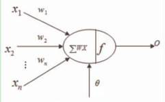
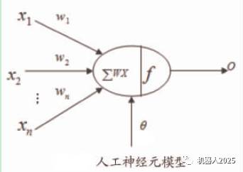
Artificial neural networks are artificial networks composed of numerous processing units that are widely interconnected, simulating the structure and functions of the brain’s neural system. These processing units are referred to as artificial neurons.. Artificial neural networks can be seen as directed graphs connected by directed weighted arcs, with artificial neurons as nodes simulating biological neurons, and directed arcs simulating the axon-synapse-dendrite pairs. The weight of the directed arcs indicates the strength of interaction between the two interconnected artificial neurons. The structure of artificial neurons is shown in the figure below:
Neural networks simulate the brain in two aspects:
(1) The knowledge acquired by neural networks is learned from the external environment.
(2) The internal connection strength of neurons, i.e., synaptic weights, is used to store the acquired knowledge.
The neural network system consists of a topological structure formed by numerous neurons that can process information transmission between different parts of the human brain. Relying on these massive numbers of neurons and their connections, the human brain can receive input information stimuli and perform nonlinear mapping processing through distributed parallel processing of interconnected neurons, thereby achieving complex information processing and reasoning tasks.
For a specific processing unit (neuron), assuming the information from other processing units (neurons) i is Xi, the interaction strength with this processing unit is the connection weight Wi, i=0,1,…,n-1, and the internal threshold of the processing unit is θ.
Then the input of this processing unit (neuron) is:  and the output of the processing unit is:
 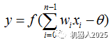 .
.
In the above formulas, xi is the input of the i-th element, wi is the interconnection weight between the i-th processing unit and this processing unit, i.e., the neuron connection weight. f is called the activation function or action function, determining the output of the node (neuron). θ indicates the threshold of hidden layer neuron nodes.
In the design and application research of artificial neural networks, three aspects typically need to be considered: the activation function of neurons, the connection forms between neurons, and the learning (training) of the network.
3. Learning Forms of Neural Networks: When constructing a neural network, the transfer function and transformation function of its neurons are already determined.
4. Working Process of Neural Networks: The working process of neural networks includes both offline learning and online judgment. During the learning process, each neuron performs rule learning, adjusts weight parameters, and fits the nonlinear mapping relationships to achieve training accuracy; the judgment phase involves the trained stable network reading input information and calculating the output results.
5. Learning Rules of Neural Networks: The learning rules of neural networks are algorithms for correcting weights, divided into associative and non-associative learning, supervised and unsupervised learning, etc. The following introduces several commonly used learning rules.
(1) Error Correction Rule: This is a supervised learning method that adjusts the network connection weights based on the error between the actual output and the expected output, ultimately resulting in the network error being less than the target function to achieve the desired result.
The error correction method relates the weight adjustment to the network output error, including the δ learning rule, Widrow-Hoff learning rule, perceptron learning rule, and error back-propagation BP (Back Propagation) learning rule.
(2) Competitive Rule: This is an unsupervised learning process where the network learns self-organizationally based on some provided learning samples without expected outputs, adjusting network weights to adapt to input sample data through competition among neurons responding to external stimulus patterns.
In unsupervised learning situations, no standard samples are given in advance; the network is directly placed in the “environment,” integrating the learning (training) and application (working) phases.
(3) Hebb Rule: This uses the activation values (activation values) between neurons to reflect changes in their connectivity, adjusting weights based on the activation values between interconnected neurons.
In Hebb learning rules, the learning signal simply equals the output of the neurons. The Hebb learning rule represents a purely feedforward, non-supervised learning approach. This learning rule has played an important role in various neural network models to date, such as training the weight matrix of linear associators using the Hebb rule.
(4) Stochastic Rule: This learning process combines randomness, probability theory, and energy functions, adjusting network parameters based on the changes in the target function (i.e., the mean square error of network output), ultimately converging to the target function value.
6. Activation Functions: In neural networks, the ability and efficiency to solve problems depend not only on the network structure but also largely on the activation functions employed by the network. The choice of activation function significantly impacts the network’s convergence speed, and different practical problems require different activation functions.
The regulation by which neurons produce output signals under the influence of input signals is given by the neuron functional function f (Activation Function), also known as the activation function or transfer function. This encompasses the process from input signals to net input, then to activation values, and finally producing output signals. It integrates the net input and the effect of the f function. The f function comes in various forms, and utilizing their different characteristics can construct neural networks with distinct functionalities.
Commonly used activation functions include:
(1) Threshold Function: This function is often referred to as the step function. When the activation function adopts the step function, the artificial neuron model becomes the MP model. At this time, the neuron’s output takes on either 1 or 0, reflecting the excitation or inhibition of the neuron.
(2) Linear Function: This function can serve as the activation function for output neurons when the output result can be any value. However, when the network is complex, the linear activation function greatly reduces the network’s convergence, thus it is generally less adopted.
(3) Logistic Sigmoid Function: The output of the logistic sigmoid function lies between 0 and 1, commonly chosen for signals required to output within the range of 0 to 1. It is the most widely used activation function in neurons.
(4) Hyperbolic Tangent Sigmoid Function: The hyperbolic tangent sigmoid function is similar to a smoothed step function, symmetric about the origin, with outputs between -1 and 1, often chosen for signals required to output within the range of -1 to 1.
7. Connection Forms Between Neurons: Neural networks are complex interconnected systems, and the interconnection patterns between units significantly impact the network’s properties and functions. There are various types of interconnection patterns.
(1) Feedforward Network: The network can be divided into several “layers,” arranged sequentially according to the order of signal transmission. Neurons in the i-th layer only accept signals from the (i-1)-th layer, with no feedback between neurons. Feedforward networks can be represented with a directed acyclic graph, as shown in the figure below:
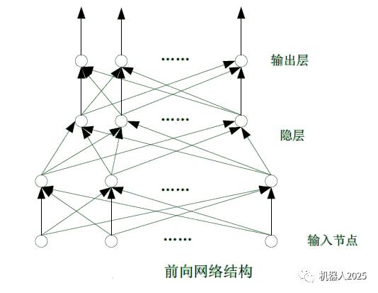
As can be seen, input nodes have no computational function; they merely represent the values of each element in the input vector. Each layer’s nodes represent computationally functional neurons, referred to as computational units. Each computational unit can have any number of inputs but only one output, which can be sent to multiple nodes as input. The input node layer is referred to as the zero layer. The nodes of each computational unit layer are sequentially referred to as the first to N-th layers, thereby forming an N-layer feedforward network. (Some also refer to the input node layer as the first layer, thus changing the N-layer network to N+1 node layer indices.)
The first node layer and output nodes are collectively referred to as the “visible layer,” while other intermediate layers are referred to as hidden layers, with these neurons called hidden nodes. The BP network is a typical feedforward network.
(2) Feedback Network: A typical feedback neural network is illustrated in the figure below:
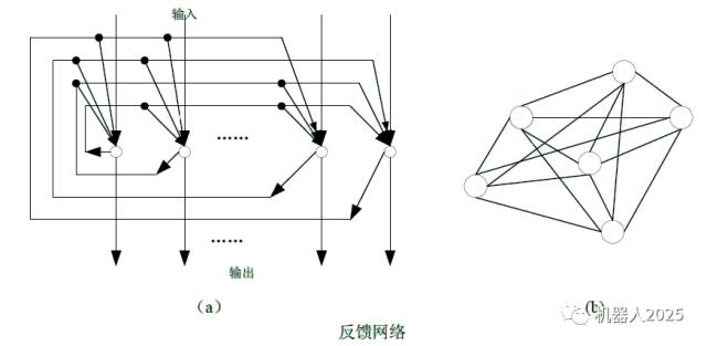
Each node represents a computational unit that simultaneously accepts external inputs and feedback inputs from other nodes, with each node also directly outputting to the outside. The Hopfield network belongs to this type. In some feedback networks, neurons not only receive external inputs and feedback inputs from other nodes but also include self-feedback. Sometimes, feedback neural networks can also be represented as a complete undirected graph, as shown in the figure. Here, the feedback from the i-th neuron to the j-th neuron is equal to the synaptic weight of the feedback from the j-th to the i-th neuron, i.e., wij=wji.
The above introduces two of the most basic structures of artificial neural networks. In fact, there are many other connection forms for artificial neural networks, such as feedforward networks with feedback from the output layer to the input layer, and multi-layer networks with feedback among nodes within the same layer or across different layers, etc.
5. Models of Artificial Neural Networks
1. Classification of Artificial Neural Networks:
By performance: continuous and discrete networks, or deterministic and stochastic networks.
By topological structure: feedforward networks and feedback networks.
Feedforward networks include adaptive linear neural networks (Adaline), single-layer perceptrons, multilayer perceptrons, BP networks, etc.
In feedforward networks, each neuron in the network accepts inputs from the previous level and outputs to the next level, with no feedback in the network, representable by a directed acyclic graph. This type of network implements transformations of signals from input space to output space, with its information processing capability deriving from the repeated compositions of simple nonlinear functions. The network structure is simple and easy to implement. Backpropagation networks are a typical feedforward network.
Feedback networks include Hopfield, Hamming, BAM, etc.
In feedback networks, there is feedback among neurons within the network, representable by an undirected complete graph. The information processing of this type of neural network involves state transformations, which can be handled using dynamical system theory. The stability of the system is closely related to the associative memory function. Both Hopfield networks and Boltzmann machines belong to this type.
By learning methods: supervised learning networks with teachers and unsupervised learning networks without teachers.
By the nature of synaptic connections: first-order linear associative networks and higher-order nonlinear associative networks.
2. Biological Neuron Model: The human brain is a high-level animal created by nature, and human thinking is accomplished by the brain, which is the concentrated embodiment of human intelligence. The cortex of the human brain contains 10 billion neurons and 60 trillion synapses, along with their connections.
3. Artificial Neural Network Model: Artificial neural networks are mathematical models that perform distributed parallel information processing by mimicking the behavioral characteristics of biological neural networks. This network relies on the complexity of the system, adjusting the relationships of interconnections among numerous internal nodes to achieve information processing objectives.
4. Perceptron Model:
The perceptron model is a type of neural network model proposed by American scholar Rosenblatt for studying the storage, learning, and cognitive processes of the brain, directing neural network research from pure theoretical exploration to practical engineering implementation.
The perceptron model proposed by Rosenblatt is a feedforward neural network with only a single layer of computational units, known as a single-layer perceptron.
The learning algorithm of the single-layer perceptron model initializes the connection weights and thresholds to small non-zero random numbers, then feeds the inputs with n connection weights into the network. If the output obtained differs significantly from the desired output, the connection weight parameters are automatically adjusted according to a certain algorithm. This process is repeated until the output meets the desired difference.
The linear inseparability problem refers to problems that cannot be expressed by a single-layer perceptron, such as the XOR problem, which was proven to be linearly inseparable by Minsky in 1969.
The number of linear inseparable functions increases rapidly with the number of input variables, far exceeding the number of linearly separable functions. In other words, the number of problems that cannot be expressed by single-layer perceptrons is far greater than the number of problems they can express.
Multilayer Perceptron: Adding one or more layers of processing units between the input part and output layer of a single-layer perceptron forms a two-layer or multi-layer perceptron.
In the multilayer perceptron model, only the connection weights of a specific layer can be adjusted, as the ideal outputs of the hidden layer neurons are unknown, making it difficult to provide an effective learning algorithm for multilayer perceptrons.
Multilayer perceptrons overcome many shortcomings of single-layer perceptrons, allowing them to solve problems that single-layer perceptrons cannot. For instance, a two-layer perceptron can solve the XOR logical operation problem.
5. Backpropagation Model:
The backpropagation model, also known as the BP model, is a learning algorithm used for feedforward multilayer networks. It is termed a learning method because it continuously modifies the connection weights between artificial neurons that make up the feedforward multilayer network, enabling the network to transform the information it inputs into the desired output. It is called a backpropagation learning algorithm because the modifications to the connection weights are based on the difference between the actual output of the network and the expected output, propagating this difference backwards layer by layer to determine the adjustments to the connection weights.
The BP algorithm’s network structure is a feedforward multilayer network. It was proposed in 1986 by Rumelhart and McClelland as a “reverse push” learning algorithm for multilayer networks. Its basic idea involves two processes: the forward propagation of signals and the backward propagation of errors. During forward propagation, input samples are fed from the input layer, processed layer by layer through hidden layers, and directed towards the output layer. If the actual output of the output layer does not match the expected output, the process transitions to the backward propagation of errors. The backward propagation of errors involves propagating the output error in a certain form through the hidden layers back to the input layer, distributing the errors to all units in each layer to obtain the error signals for each layer’s units, which serve as the basis for correcting the weights of each unit. This process of signal forward propagation and error backward propagation is iterative. The weight adjustment process continues until the network output error is reduced to an acceptable level or until a predetermined number of learning iterations is reached.
The learning algorithm of the backpropagation network aims to adjust the connection weights of the network so that the adjusted network can produce the expected output for any given input.
The learning process consists of forward propagation and backward propagation.
Forward propagation is used for computing the feedforward network, i.e., calculating the output result for a specific input information after processing through the network.
Backward propagation is used to propagate errors layer by layer, modifying the connection weights between neurons to ensure that the network’s output meets the desired error requirements after computation.
The learning process of the BP algorithm is as follows:
(1) Select a set of training samples, each consisting of input information and expected output.
(2) Take a sample from the training sample set and input the information into the network.
(3) Calculate the outputs of each layer’s nodes after processing through the neurons.
(4) Calculate the error between the actual output of the network and the expected output.
(5) Backtrack from the output layer to the first hidden layer, adjusting the connection weights of the neurons in the network according to a principle that promotes error reduction.
(6) Repeat steps (3) to (5) for each sample in the training sample set until the error for the entire training sample set meets the requirements.
In the above learning process, step (5) is the most important, as determining a principle for adjusting connection weights to promote error reduction is a critical challenge that the BP learning algorithm must address.
The advantages and disadvantages of the BP algorithm:
Advantages: The theoretical foundation is solid, the derivation process is rigorous, the physical concepts are clear, and it has good generality. Therefore, it is currently the best algorithm for training feedforward multilayer networks.
Disadvantages: (1) The convergence speed of this learning algorithm is slow; (2) There is no theoretical guidance for selecting the number of hidden nodes in the network; (3) From a mathematical perspective, the BP algorithm is a gradient descent method, which may lead to local minima problems. When local minima occur, the error may seem acceptable, but the solution obtained may not be the true solution to the problem, indicating that the BP algorithm is incomplete.
Limitations of the BP algorithm:
(1) There are regions on the error surface that are flat, where the error is not sensitive to weight changes, leading to slow error reduction and prolonged adjustment time, affecting convergence speed. In such cases, the gradient of the error changes is small, and even if the weight adjustments are significant, the error still decreases slowly. This situation is often related to excessive net inputs to each node.
(2) Multiple local minima exist. The error surface in two-dimensional weight space shows numerous convex and concave regions, with the low concave parts representing local minima of the error function. It can be imagined that the error surface in multi-dimensional weight space is even more complex, containing many local minima, all characterized by gradients of zero. The weight adjustment of the BP algorithm relies on the gradient descent of the error; when the gradient is zero, the BP algorithm cannot discern the nature of the local minima, causing training to become trapped in a local minimum and unable to converge to the specified error.
Improvements to the BP algorithm: The flat areas of the error surface lead to slow error reduction, extended adjustment times, and increased iterations, thereby affecting convergence speed. The presence of multiple local minima can cause network training to become trapped in local minima, preventing convergence to the specified error. These two issues are inherent flaws in the standard BP algorithm.
In response, many scholars at home and abroad have proposed numerous improved algorithms, with several typical improvements including:
(1) Adding a momentum term: The standard BP algorithm adjusts weights based solely on the gradient descent direction of the error at time t, without considering the gradient direction from previous moments, often causing oscillations and slow convergence during training. To improve training speed, a momentum term can be added to the weight adjustment formula. Most BP algorithms incorporate a momentum term, making BP algorithms with momentum terms a new standard algorithm.
(2) Variable learning rate backpropagation algorithm (VLBP): The error surface of multilayer networks is not a quadratic function. The shape of the surface varies across different regions of parameter space. The learning speed can be adjusted during learning to enhance convergence speed. The challenge lies in determining when and how to change the learning speed. There are various methods for adjusting the learning speed in the VLBP algorithm.
(3) Adaptive adjustment of learning rates: The variable learning rate VLBP algorithm requires setting multiple parameters, and the algorithm’s performance is often sensitive to changes in these parameters, making it cumbersome to handle. Here, a simple adaptive adjustment algorithm for the learning rate is provided. The adjustment of the learning rate, also known as the step size, only relates to the total error of the network. In standard BP, it is a constant, but in practice, it is challenging to specify an optimal learning rate that is suitable throughout the process. As seen in the error surface, if η is too small in flat regions, the number of training iterations increases, while in regions of rapid error change, if η is too large, it may overshoot narrow “pits,” causing oscillations and increasing iteration times. To accelerate the convergence process, it is best to adaptively adjust the learning rate η, making it larger when necessary and smaller when needed. For instance, it can be adjusted based on the total error of the network.
(4) Introducing steepness factors – preventing saturation: Flat areas on the error surface cause slow weight adjustments. The reason for this slow adjustment is due to the saturation characteristics of the S transfer function. If, after entering a flat area, efforts are made to compress the net input of the neurons to keep their outputs from entering the saturation region of the transfer function, the shape of the error function can be altered, allowing adjustments to escape the flat area. The specific approach to achieving this idea is to introduce a steepness factor into the transfer function.
The general principles for designing BP neural networks: Most designs are based on user experience to structure the network, functional functions, learning algorithms, samples, etc.
[1] BP network parameter design
(1) Determining input and output parameters for BP networks
A. Selection of input variables:
a. Input variables must be those that significantly influence the output and can be detected or extracted;
b. Input variables should be minimally correlated or uncorrelated. Input and output variables can be categorized into two types: numerical variables and linguistic variables. Numerical variables can be continuous or discrete. For example, common temperature, pressure, voltage, current, etc., are continuous variables; linguistic variables are concepts expressed in natural language, such as red, green, blue; male, female; large, medium, small; on, off, bright, dark, etc. In general, linguistic variables need to be converted into discrete variables during network processing.
c. Representation and extraction of input variables: In most cases, the input variables directly fed into the neural network cannot be obtained directly and often require signal processing and feature extraction techniques to derive parameters reflecting their characteristics from raw data.
B. Selection and representation of output variables:
a. Output variables generally represent the functional objectives that the system aims to achieve, such as category attribution in classification problems;
b. Output variables can be numerical or linguistic variables;
(2) Designing the training sample set
The performance of the network is closely related to the samples used for training, and designing a good training sample set requires attention to both sample size and quality.
A. Determining the number of samples: Generally, the more samples (n), the more accurately the training results reflect the underlying patterns. However, obtaining samples often poses challenges, and once the number of samples reaches a certain level, improving the network’s accuracy becomes difficult.
Selection principle: The larger the network scale, the more complex the network mapping relationships, and the more samples are needed. Generally, the number of training samples is 5 to 10 times the total number of network connection weights, but achieving this requirement is often challenging.
B. Selection and organization of samples:
a. Samples must be representative, ensuring balance among sample categories;
b. The organization of samples should ensure that different categories of samples are input in a crosswise manner;
c. Testing the network’s training involves evaluating whether it possesses good generalization capabilities. Testing methods: Do not use data from the training sample set for testing. Typically, the collected usable samples are randomly divided into two parts: one part for training and the other for testing. If the training sample error is minimal while the error for the testing sample is significant, generalization capability is poor.
(3) Designing initial weights
The initialization of network weights determines where the network training begins on the error surface, making the initialization method crucial for shortening training time.
The action function of neurons is symmetrical concerning coordinates. If the net inputs of each node are near zero, the outputs will be centered in the action function, far from the saturation area, and in the most sensitive region of its variation, thus accelerating network learning. To keep the initial net inputs of each node near zero, the following two methods are commonly used:
A. Use sufficiently small initial weights;
B. Ensure the initial number of weights set to +1 and -1 are equal.
[2] Designing BP network structure parameters
Hidden layer structure design
(1) Designing the number of hidden layers: Theoretical proof indicates that a feedforward network with a single hidden layer can map all continuous functions, while two hidden layers are only necessary when learning discontinuous functions. Thus, in general, a maximum of two hidden layers is required. The common approach is to start with one hidden layer, and if a single hidden layer with many nodes still does not improve network performance, an additional hidden layer can be added. The most commonly used BP neural network structure is a three-layer structure, consisting of an input layer, output layer, and one hidden layer.
(2) Designing the number of hidden layer nodes: The number of hidden layer nodes significantly impacts the performance of the neural network. If the number of hidden layer nodes is too few, the learning capacity is limited, insufficient to store all the patterns contained in the training samples; if too many hidden layer nodes are present, it not only increases training time but also risks storing non-pattern elements like interference and noise, consequently reducing generalization capability. The common method is trial and error.
6. Hopfield Model:
The Hopfield model was proposed by Hopfield in 1982 and 1984, consisting of two neural network models. The 1982 model is discrete, while the 1984 model is continuous, but both are feedback network structures.
The discrete Hopfield network has two working modes:
(1) Serial mode, where at any moment t, only one neuron i changes state while the rest remain unchanged.
(2) Parallel mode, where at any moment t, some or all neurons simultaneously change state.
Regarding the stability of the discrete Hopfield network, Cohen and Grossberg provided a proof in 1983. Hopfield et al. further demonstrated that as long as the matrix formed by the connection weights is a symmetric matrix with non-negative diagonal elements, the network will exhibit serial stability.
The Hopfield recursive network was proposed by American physicist J.J. Hopfield in 1983. The Hopfield network can be categorized into discrete and continuous types based on the numerical forms of its input and output, namely: Discrete Hopfield Neural Network (DHNN) and Continuous Hopfield Neural Network (CHNN).
DHNN Structure: It is a single-layer fully feedback network with n neurons. Each neuron receives feedback information from all other neurons via connection weights, allowing any neuron’s output to be controlled by the outputs of all neurons, thus enabling mutual constraints among neurons.
Design principles of DHNN: The distribution of attractors is determined by the network’s weights (including thresholds), with the core design of attractors focusing on how to design a suitable weight set. To ensure that the designed weights meet the requirements, the weight matrix should adhere to the following conditions: (1) To guarantee convergence during asynchronous operation, W should be a symmetric matrix; (2) To ensure convergence during synchronous operation, W should be a non-negative definite symmetric matrix; (3) To ensure that the given sample is an attractor of the network and has a certain attractor domain.
In specific designs, different methods can be employed: (1) Simultaneous equations method; (2) Outer product and sum method.
CHNN: In the continuous Hopfield neural network, all neurons update in parallel over time t, with the network state continuously changing over time.
The main functions of Hopfield networks are closely related to their practical applications. Their primary functions include:
(1) Associative memory: There is no one-to-one mapping relationship between the elements of input-output patterns, and the dimensions of input-output patterns do not need to be the same; during associative memory, by providing partial information of the input pattern, a complete output pattern can be inferred. This indicates fault tolerance.
(2) CHNN’s optimization computation function.
Using the Hopfield neural network to solve optimization problems generally involves the following steps:
A. Problem analysis: The network output corresponds to the solution of the problem.
B. Constructing the network energy function: A suitable network energy function is constructed so that its minimum value corresponds to the optimal solution of the problem.
C. Designing the network structure: The energy function is compared with the standard form to determine the weight matrix and bias current.
D. Establishing the electronic circuit of the network based on the network structure and running it to achieve steady state – optimization solution or computer simulation.
7. BAM Model
The associative memory function of neural networks can be divided into two types: self-associative memory and hetero-associative memory. The Hopfield neural network belongs to the self-associative memory category. The Bidirectional Associative Memory (BAM), proposed by Kosko B. in 1988, belongs to the hetero-associative memory category. BAM includes discrete, continuous, and adaptive forms.
8. CMAC Model
BP neural networks, Hopfield neural networks, and BAM bidirectional associative memory neural networks are categorized as feedforward and feedback neural networks primarily based on their structures. If categorized based on their function approximation capabilities, neural networks can be divided into global approximation networks and local approximation networks. When one or more adjustable parameters (weights and thresholds) of a neural network influence any output at every point in the input space, the neural network is termed a global approximation network; multilayer feedforward BP networks are typical examples of global approximation networks.
CMAC networks have three characteristics:
(1) As a type of associative neural network, its associations have local generalization capabilities (or generalization ability), meaning similar inputs will produce similar outputs, while distant inputs will yield independent outputs;
(2) For each output of the network, only a few neurons’ corresponding weights influence it, determined by the inputs;
(3) The input-output relationship of each neuron in CMAC is linear, but overall, it can be viewed as a tabular system expressing nonlinear mappings. Since learning in CMAC networks occurs only in the linear mapping portion, simple δ algorithms can be employed, resulting in much faster convergence speeds than BP algorithms, without local minimum issues. CMAC was initially used to solve joint movements of robotic arms and subsequently applied in robot control, pattern recognition, signal processing, and adaptive control.
9. RBF Model
For local approximation neural networks, besides CMAC networks, commonly used models include Radial Basis Function (RBF) networks and B-spline networks. Radial Basis Function (RBF) neural networks, proposed by J. Moody and C. Darken in the late 1980s, utilize traditional strict interpolation methods in multi-dimensional space to some extent.
The conventional learning algorithm for RBF networks generally includes two different stages:
(1) The stage of determining the centers of the hidden layer radial basis functions. Common methods include randomly selecting fixed centers and self-organizing selection methods for centers.
(2) The stage of learning and adjusting the weights of radial basis functions. Common methods include supervised selection of centers and regularized strict interpolation methods.
10. SOM Model
Professor Kohonen from Helsinki University in Finland proposed a Self-Organizing Feature Map (SOM), also known as a Kohonen network. Kohonen believed that when a neural network receives external input patterns, it will be divided into different corresponding regions, each responding to input patterns with different features, and this process is completed automatically. The SOM network is proposed based on this understanding, exhibiting characteristics similar to the self-organizing properties of the human brain.
Self-organizing neural network structure
(1) Definition: A self-organizing neural network is an unsupervised learning network. It automatically alters network parameters and structure by seeking the inherent laws and essential properties within samples.
(2) Structure: Hierarchical structure with a competitive layer. Typical structure: input layer + competitive layer.
Input layer: Accepts external information and transmits input patterns to the competitive layer, serving an “observational” role.
Competitive layer: Responsible for “analyzing and comparing input patterns, finding patterns, and classifying them.
The principle of self-organizing neural networks
(1) Classification and similarity of input patterns: Classification involves allocating input patterns to their respective classes under the guidance of category knowledge and other teacher signals. Unsupervised classification is referred to as clustering, where the goal is to group similar pattern samples together while separating dissimilar ones.
(2) Similarity measurement: The similarity of input pattern vectors in neural networks can be measured using the distance between vectors. Common methods include Euclidean distance and cosine methods.
(3) Competitive learning principle: The physiological basis of competitive learning rules is the lateral inhibition phenomenon of nerve cells: when one nerve cell is excited, it inhibits surrounding nerve cells. The strongest inhibition occurs when only the winning neuron remains active, a practice known as “winner-take-all” (WTA). The competitive learning rule is derived from the lateral inhibition phenomenon of nerve cells. Its learning steps are: A. Normalize the vector; B. Find the winning neuron; C. Adjust network output and weights; D. Re-normalize.
The topological structure of the SOM network: The SOM network consists of two layers: the input layer and the output layer.
(1) Input layer: Gathers external information into the output layer neurons through weight vectors. The input layer is structured similarly to the BP network, with the number of nodes matching the dimensionality of the samples.
(2) Output layer: The output layer is also a competitive layer. Its neurons can be arranged in multiple forms, including one-dimensional linear arrays, two-dimensional planar arrays, and three-dimensional grid arrays. The most typical structure is two-dimensional, resembling the brain cortex.
Each neuron in the output layer is laterally connected to its surrounding neurons, arranged in a checkerboard pattern; the input layer consists of a single layer of neurons.
The adjustment domain of SOM weights
The algorithm used by SOM networks is called the Kohonen algorithm, which is an improvement based on the winner-take-all (WTA) learning rule. The main difference lies in the way the adjustment of weight vectors occurs. In WTA, lateral inhibition is a “kill” method, where only the winning neuron can adjust its weight, while other neurons cannot adjust. In the Kohonen algorithm, the winning neuron influences its neighboring neurons from near to far, transitioning from excitation to inhibition. In other words, not only does the winning neuron adjust its weight, but nearby neurons also adjust their weight vectors to varying degrees.
Running principles of SOM networks
The operation of SOM networks consists of two phases: training and working. During the training phase, the network randomly inputs samples from the training set. For a specific input pattern, one node in the output layer will generate the maximum response and win. However, at the beginning of training, it is uncertain which node in the output layer will respond most strongly to which input pattern.
11. CPN Model
In 1987, American scholar Robert Hecht-Nielsen proposed the Counter-Propagation Networks (CPN). CPN was initially used to implement sample selection matching systems. It can store binary or analog value patterns, making it suitable for associative storage, pattern classification, function approximation, and data compression. Compared to BP networks, CPN trains much faster, requiring only about 1% of the time needed by BP networks. However, its application scope is relatively narrow due to its performance limitations.
The self-organizing mapping proposed by Kohonen consists of four parts, including a neuron array (which forms the Kohonen layer of CPN), a comparison selection mechanism, local interconnections, and an adaptive process. In practice, this layer performs the function of classifying inputs. Thus, it can execute unsupervised learning to extract classification information contained within the sample set.
The Grossberg layer primarily implements class representation. Its training process involves matching input vectors with corresponding output vectors. These vectors can be binary or continuous. Once the network completes training, it can provide a corresponding output for a given input. The network’s generalization capability indicates that when it encounters an incomplete or imperfect input, as long as the “noise” falls within a limited range, CPN can still produce a correct output. This is because the Kohonen layer can determine the classification to which the noisy input belongs, while the corresponding Grossberg layer provides the representation of that classification. Overall, the network exhibits a generalized capability, making it applicable in areas such as pattern recognition, pattern completion, and signal processing.
12. ART Model
In 1976, Professor Carpenter G.A. from Boston University proposed the Adaptive Resonance Theory (ART). Subsequently, Carpenter G.A. collaborated with his student Grossberg S. to propose ART neural networks.
After years of research and development, several basic forms of ART networks have emerged:
(1) ART1 neural network: Handles bipolar and binary signals;
(2) ART2 neural network: An extension of ART1 for processing continuous analog signals;
(3) ART integrated systems: Combining ART1 and ART2, the system possesses recognition, reinforcement, and recall functions, known as the 3R (Recognition, Reinforcement, Recall) function.
(4) ART3 neural network: A hierarchical search model that integrates the functions of the first two structures and expands the two-layer neural network into an arbitrary multi-layer neuron network. Due to the incorporation of the biological electrochemical reaction mechanisms of biological neurons into the ART3 model, it possesses strong functionality and extensibility.
13. Quantum Neural Networks
The concept of quantum neural networks emerged in the late 1990s, attracting attention from scientists across various fields. Different directions of exploration have been proposed, showcasing the immense potential of quantum neural network research. The main research directions can be summarized as follows:
(1) Quantum neural networks construct quantum computers using the connection ideas of neural networks, studying issues in quantum computing through neural network models;
(2) Quantum neural networks are constructed on the foundation of quantum computers or quantum devices, fully utilizing the characteristics of quantum computing, such as ultra-high speed, ultra-parallelism, and exponential capacity, to improve the structure and performance of neural networks;
(3) Quantum neural networks serve as a hybrid intelligent optimization algorithm implemented on traditional computers, improving traditional neural networks by introducing concepts and methods from quantum theory (e.g., state superposition, the multiverse perspective, etc.) to establish new network models and enhance the structure and performance of traditional neural networks;
(4) Research based on brain science and cognitive science.
The above content is primarily extracted from:
1. “Principles and Applications of Artificial Neural Networks,” 2006, Science Press
2. “Research on Neural Network Email Classification Algorithms,” 2011, Master’s Thesis, University of Electronic Science and Technology of China
3. “Principles, Classification, and Applications of Artificial Neural Networks,” 2014, Journal, Science and Technology Information
Reprinted from Robotics 2025
Press the QR code below for free subscription!
How to Join the Society
Register as a Society Member:
Individual Members:
Follow the Society’s WeChat: China Command and Control Society (c2_china), reply with “Individual Member” to obtain the membership application form. Fill out the application form as required. If there are any questions, please leave a message in the public account. Payment of membership fees via Alipay can only be made after passing the society’s review.
Institutional Members:
Follow the Society’s WeChat: China Command and Control Society (c2_china), reply with “Institutional Member” to obtain the membership application form. Fill out the application form as required. If there are any questions, please leave a message in the public account. Payment of membership fees can only be made after passing the society’s review.
Recent Activities of the Society
1. 2016 Annual “CICC Science and Technology Award Ceremony”
Meeting Time: March 28, 2017
2. CICC Corporate Member Exchange Meeting
Meeting Time: (Specific time will be detailed in subsequent notices)
3. 2017 First National Military Chess Simulation Competition
June 2017
Long press the QR code below to follow the society’s WeChat

Thank you for your attention