In-Depth Time Series Prediction Using LSTM Neural Networks

Click on the top "Xiaobai Learns Vision", select to add "Star" or "Pin"
Heavyweight content delivered at the first time

Introduction
RNN (Recurrent Neural Network) is an artificial neural network with nodes oriented in a circular connection. Unlike feedforward neural networks, RNNs can utilize internal memory to process any sequential input series, meaning they learn not only from the current moment’s information but also rely on previous sequence information, which gives them significant advantages in tasks like speech recognition and language translation. There are many variants of RNN now, commonly used ones include LSTM, Seq2Seq LSTM, and other variants such as Transformer models with Attention mechanisms. Although these variants may seem complex in principle and structure, as long as one has a solid foundation in mathematics and computer science, understanding one model thoroughly makes the rest easier to grasp.
This article will provide a highly condensed introduction to the knowledge within LSTM (including feedforward derivation and chain rule), followed by the establishment of a time series model and optimization of the model, ultimately evaluating the model and comparing it with ARIMA or ARIMA-GARCH models.
In-Depth Time Series Prediction Using LSTM Neural Networks
1 RNN Neural Network Underlying Logic Introduction
(Note: All model explanation diagrams below are sourced from Baidu Images)
1.1 Input Layer, Hidden Layer, and Output Layer
In-Depth Time Series Prediction Using LSTM Neural Networks
▲ Figure 1
From the above Figure 1, assume that is the batch input at the th position in the sequence (where is the number of samples, and is the feature dimension of the samples), corresponding to the hidden layer state (where is the length of the hidden layer), and the final output is (where is the dimension of the output vector, i.e., how many elements the output vector contains!). When calculating at time , we have the formula:
In-Depth Time Series Prediction Using LSTM Neural Networks
Here, is a specific activation function, is the weight to be learned, and is the bias value to be learned. Similarly, the output result is: Parameter explanations are as above!
1.2 Definition of Loss Function
Based on the nature of the error function, for regression problems, most are established based on distance forms such as mean square error or absolute error functions. For classification problems, we generally choose functions like cross-entropy!
At time , there is an error , where is the true value, and is the predicted value. Over the entire time length , we have , our goal is to update all parameters and to minimize .
1.3 Gradient Descent and Chain Rule Derivation
The derivation here is relatively complex. To help everyone understand the model’s concept rather than purely academic research, only key points will be introduced! Also, the activation function is simplified!
For parameter , the classic gradient descent format is: , according to calculus knowledge, we know that the chain rule formula is: if , then can be expressed as the chain derivation process!
Now, let’s derive the chain derivation results for various functions. For any output at time , it is easy to know from the definition of the loss function: , then for the update of , it takes steps to reach , summing gives:
In-Depth Time Series Prediction Using LSTM Neural Networks
For the terminal time , we can easily have:

In-Depth Time Series Prediction Using LSTM Neural Networks
However, for the time <, the derivation for the hidden layer is more complex due to the temporal relationship, so we have:
In-Depth Time Series Prediction Using LSTM Neural Networks
Similarly, it is easy to solve:
In-Depth Time Series Prediction Using LSTM Neural Networks

2 Explanation of Gradient Vanishing (Exploding) Principle

Generally, RNN models will face the problem of gradient vanishing (exploding) due to the chain rule, so we need to develop new variants to solve this problem. But where exactly is this gradient issue? Upon careful inspection during the derivation process of the previous section’s (*) formula, for hidden layer derivation, we can rewrite the (*) formula to obtain:
In-Depth Time Series Prediction Using LSTM Neural Networks
We then push one step further and derive it to time , ultimately obtaining through mathematical induction:
In-Depth Time Series Prediction Using LSTM Neural Networks
From this formula, we know that when and increase or decrease, due to the power calculation, the result will suddenly increase or tend to vanish! Thus, the general introduction of RNN theory ends here. For those who want to understand in detail, please refer to relevant papers.

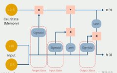
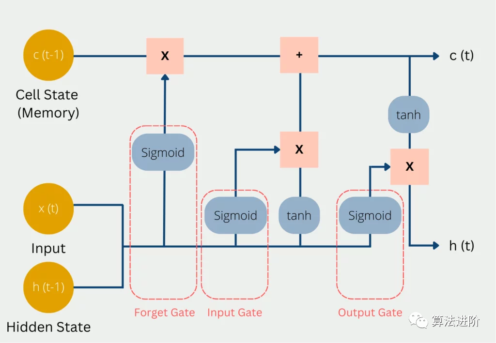
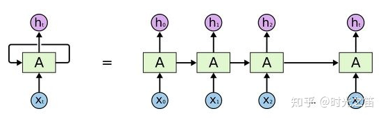
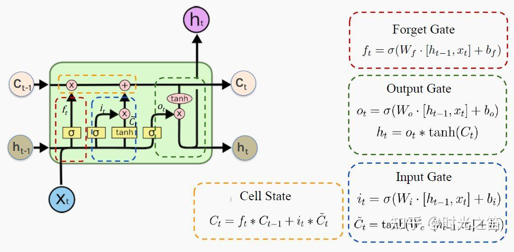
3 Introduction to LSTM Underlying Theory

In order to better capture dependencies with large intervals in time series, the Long Short-Term Memory Network (LSTM) based on gated control was born!
In-Depth Time Series Prediction Using LSTM Neural Networks
▲ Figure 2
The so-called “gate” structure is used to remove or add information to the cell state. The cell state here is the core, belonging to the hidden layer, similar to a conveyor belt, running along the entire chain, making it easy for information to flow and remain unchanged!
The above Figure 2 vividly depicts the core “three-gate structure” of LSTM. The red circle represents the so-called forget gate, which at time is represented by the following formula (if we truly understand the logic of RNN, understanding LSTM will become relatively easy):
In-Depth Time Series Prediction Using LSTM Neural Networks
The blue circle input gate has
In-Depth Time Series Prediction Using LSTM Neural Networks
The green circle output gate has
In-Depth Time Series Prediction Using LSTM Neural Networks
Similarly, the parameters and involved above are those that need to be updated through the chain rule! Thus, the final formula for calculating cell information in the yellow circle:
In-Depth Time Series Prediction Using LSTM Neural Networks
Where
In-Depth Time Series Prediction Using LSTM Neural Networks
The hyperbolic tangent function involved here is generally fixed, so why go through all this trouble and have so much information control? Of course, it is to update the cell value in order to obtain the next hidden layer value:
In-Depth Time Series Prediction Using LSTM Neural Networks
3.1 Significance of Sigmoid Activation Function
When the activation function is chosen as sigmoid, which belongs to the range of 0~1, the forget gate is approximately equal to 1, and the input gate is approximately equal to 0, which means is not updated, thus the past cell information is retained until now, solving the gradient vanishing problem.
Similarly, the output gate can be approximately equal to 1 or approximately equal to 0, when it is approximately equal to 1, the cell information will be passed to the hidden layer; when it is approximately equal to 0, the cell information will only be retained. Thus, all parameters are updated and continue to proceed…

PS: Beginners may find it painful to see so many symbols, but the logic goes from simple to complex. Thoroughly understanding RNN helps with understanding later models. I have also omitted many details here; the overall model framework is like this, which is completely sufficient for understanding how the model works. As for how it was derived and the more detailed derivation process, due to the author’s limited ability, please refer to relevant RNN papers and engage in more discussions and learning!

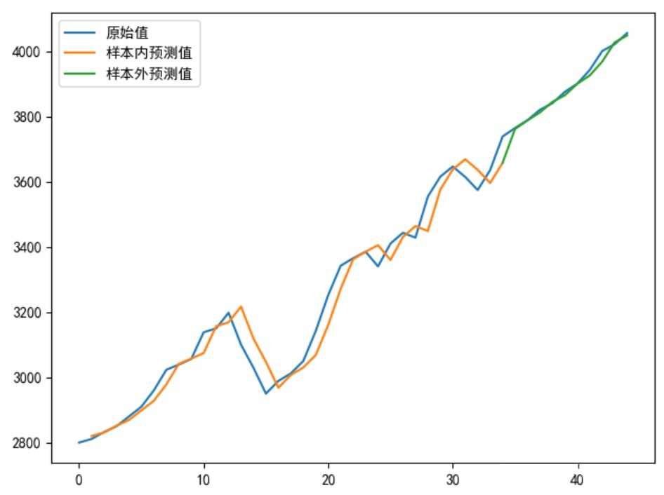
4 What to Do About “Right Shift” in Model Prediction!

To conduct comparison experiments, we will also select the actual sales data corresponding to the previous time series article! We will build our own LSTM network for time series prediction based on the Keras module.
In-Depth Time Series Prediction Using LSTM Neural Networks
▲ Figure 3: Actual Sales Data
4.1 Constructing a General LSTM Model, When We Choose a Step Length of 1, the Results Are as Follows
In-Depth Time Series Prediction Using LSTM Neural Networks
▲ Figure 4
Normally, establishing an LSTM model prediction will exhibit a right shift phenomenon in predicted values, even though R2 or MSE are quite good, the established model is actually ineffective!
4.2 Causes and Improvements
When the model tends to take the true value from the previous moment as the predicted value for the next moment, it leads to a lag between the two curves, meaning the true value curve lags behind the predicted value curve, as shown in Figure 4. The reason for this is that the sequence has autocorrelation; for example, first-order autocorrelation refers to the correlation between the current value and its previous value. Therefore, if a sequence has first-order autocorrelation, what the model learns is first-order correlation. The way to eliminate autocorrelation is to perform differencing, meaning we can use the difference between the current moment and the previous moment as our regression target.
Moreover, from the previous article’s white noise test, it was also found that this sequence indeed has strong autocorrelation! As shown in Figure 5.
In-Depth Time Series Prediction Using LSTM Neural Networks
▲ Figure 5

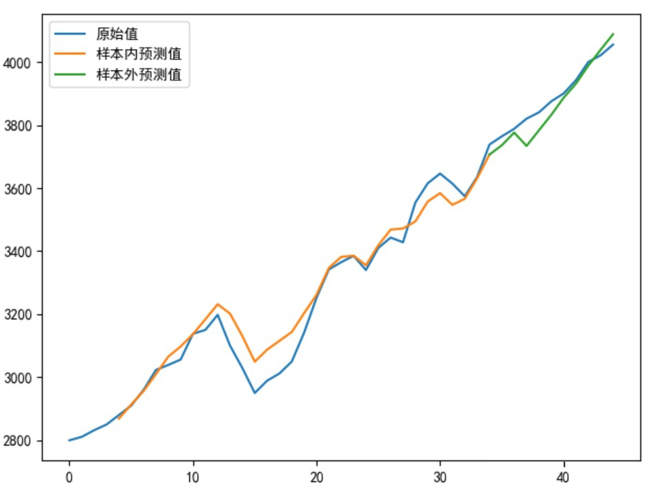
5 Improved Model Output

Let’s take a look at the final output results of the model:
In-Depth Time Series Prediction Using LSTM Neural Networks
▲ Figure 6: LSTM Results
5.1 Optimal Output Results Under Classic Time Series Models
The principle of order determination and modeling analysis of the ARIMA model:
https://zhuanlan.zhihu.com/p/417232759
In-Depth Time Series Prediction Using LSTM Neural Networks
▲ Figure 7: ARIMA Results
The global MSE of this result is 4401.02, which is greater than the MSE of the LSTM network at 2521.30. This shows that after optimizing the LSTM model, the time series modeling is superior to ARIMA or ARIMA-GARCH to some extent!
The prediction theory of LSTM differs from ARIMA; LSTM primarily predicts lagged data based on sliding window data training, where the cell mechanism reduces some parameters due to weight sharing. The ARIMA model, on the other hand, is based on autoregressive theory, establishing models related to its past. Both share the commonality of effectively utilizing sequential data, and through continuous iterations can predict indefinitely, but the prediction model is still effective for short-term predictions; long-term predictions will inevitably lead to significant deviations and may result in predicted values tending to remain unchanged.

6 Final Code

from keras.callbacks import LearningRateScheduler
from sklearn.metrics import mean_squared_error
from keras.models import Sequential
import matplotlib.pyplot as plt
from keras.layers import Dense
from keras.layers import LSTM
from keras import optimizers
import keras.backend as K
import tensorflow as tf
import pandas as pd
import numpy as np

plt.rcParams['font.sans-serif']=['SimHei']##Chinese garbled problem!
plt.rcParams['axes.unicode_minus']=False#Horizontal axis negative sign display problem!

###Initialize parameters
my_seed = 369#Random seed
 tf.random.set_seed(my_seed)##Running tf can truly fix the random seed

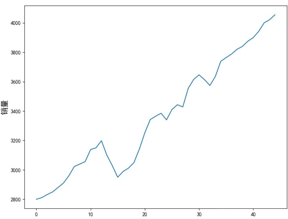
sell_data = np.array([2800,2811,2832,2850,2880,2910,2960,3023,3039,3056,3138,3150,3198,3100,3029,2950,2989,3012,3050,3142,3252,3342,3365,3385,3340,3410,3443,3428,3554,3615,3646,3614,3574,3635,3738,3764,3788,3820,3840,3875,3900,3942,4000,4021,4055])
num_steps = 3##Take sequence step length
test_len = 10##Test set length
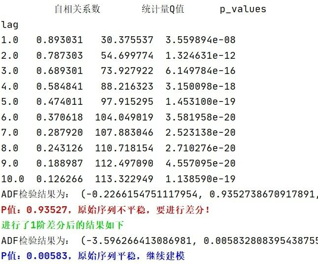
S_sell_data = pd.Series(sell_data).diff(1).dropna()##Differencing
revisedata = S_sell_data.max()
sell_datanormalization = S_sell_data / revisedata##Data normalization

##Data shape transformation, very important!!
def data_format(data, num_steps=3, test_len=5):
    # Group according to test_len
    X = np.array([data[i: i + num_steps]
                  for i in range(len(data) - num_steps)])
    y = np.array([data[i + num_steps]
                  for i in range(len(data) - num_steps)])

    train_size = test_len
    train_X, test_X = X[:-train_size], X[-train_size:]
    train_y, test_y = y[:-train_size], y[-train_size:]
    return train_X, train_y, test_X, test_y

transformer_selldata = np.reshape(pd.Series(sell_datanormalization).values,(-1,1))
train_X, train_y, test_X, test_y = data_format(transformer_selldata, num_steps, test_len)
print('\033[1;38mOriginal sequence dimension information:%s;Converted training set X data dimension information:%s,Y data dimension information:%s;Test set X data dimension information:%s,Y data dimension information:%s\033[0m'%(transformer_selldata.shape, train_X.shape, train_y.shape, test_X.shape, test_y.shape))

def buildmylstm(initactivation='relu',ininlr=0.001):

    nb_lstm_outputs1 = 128#Number of neurons
    nb_lstm_outputs2 = 128#Number of neurons
    nb_time_steps = train_X.shape[1]#Time series length
    nb_input_vector = train_X.shape[2]#Input sequence
    model = Sequential()
    model.add(LSTM(units=nb_lstm_outputs1, input_shape=(nb_time_steps, nb_input_vector),return_sequences=True))
    model.add(LSTM(units=nb_lstm_outputs2, input_shape=(nb_time_steps, nb_input_vector)))
    model.add(Dense(64, activation=initactivation))
    model.add(Dense(32, activation='relu'))
    model.add(Dense(test_y.shape[1], activation='tanh'))

    lr = ininlr
    adam = optimizers.adam_v2.Adam(learning_rate=lr)
    def scheduler(epoch):##Write learning rate change function
        # Reduce the learning rate to 1/10 of the original every epoch
        if epoch % 100 == 0 and epoch != 0:
            lr = K.get_value(model.optimizer.lr)
            K.set_value(model.optimizer.lr, lr * 0.1)
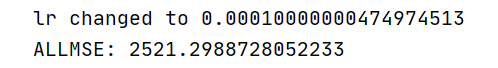
            print('lr changed to {}'.format(lr * 0.1))
        return K.get_value(model.optimizer.lr)
    model.compile(loss='mse', optimizer=adam, metrics=['mse'])##Based on the nature of the loss function, regression modeling generally uses "distance error" as the loss function, while classification generally selects "cross-entropy" loss function
    reduce_lr = LearningRateScheduler(scheduler)
    ###Data set is small, all participate, epochs generally proportional to batch_size
    ##callbacks: Callback function, calling reduce_lr
    ##verbose=0: Non-redundant printing, that is, do not print the training process
    batchsize = int(len(sell_data) / 5)
    epochs = max(128,batchsize * 4)##Minimum loop count 128
    model.fit(train_X, train_y, batch_size=batchsize, epochs=epochs, verbose=0, callbacks=[reduce_lr])

    return model

def prediction(lstmmodel):

    predsinner = lstmmodel.predict(train_X)
    predsinner_true = predsinner * revisedata
    init_value1 = sell_data[num_steps - 1]##Due to the existence of step length relationship, here the starting point is num_steps
    predsinner_true = predsinner_true.cumsum()  ##Differencing restoration
    predsinner_true = init_value1 + predsinner_true

    predsouter = lstmmodel.predict(test_X)
    predsouter_true = predsouter * revisedata
    init_value2 = predsinner_true[-1]
    predsouter_true = predsouter_true.cumsum()  ##Differencing restoration
    predsouter_true = init_value2 + predsouter_true
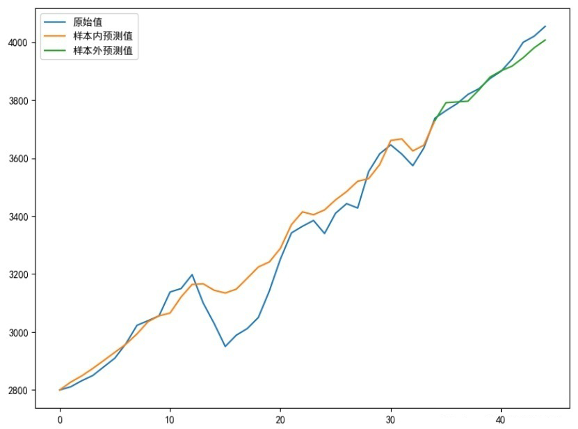
    # Plotting
    plt.plot(sell_data, label='Original Value')
    Xinner = [i for i in range(num_steps + 1, len(sell_data) - test_len)]
    plt.plot(Xinner, list(predsinner_true), label='Sample Inner Predicted Value')
    Xouter = [i for i in range(len(sell_data) - test_len - 1, len(sell_data))]
    plt.plot(Xouter, [init_value2] + list(predsouter_true), label='Sample Outer Predicted Value')
    allpredata = list(predsinner_true) + list(predsouter_true)
    plt.legend()
    plt.show()

    return allpredata

mymlstmmodel = buildmylstm()
presult = prediction(mymlstmmodel)

def evaluate_model(allpredata):

    allmse = mean_squared_error(sell_data[num_steps + 1:], allpredata)
    print('ALLMSE:',allmse)

evaluate_model(presult)
The above code can be copied directly for use, and I have annotated the key parts. If there are unclear places, please feel free to communicate; perhaps this model could also be optimized, so feel free to discuss. For LSTM modeling, data dimension transformation is a necessary step; everyone should understand it thoroughly!

7 Summary

No model is omnipotent; the key is to have the ability to discover and solve problems.
Modeling with small data is often more difficult than with large data and requires more thought.
For deep model learning, I strongly recommend having a general understanding of the model’s connotation and principles. If conditions permit, one could even derive or simply implement the gradient descent algorithm and loss function construction, etc.; otherwise, it is difficult to solve real problems.
Download 1: OpenCV-Contrib Extension Module Chinese Version Tutorial

Reply "OpenCV Extension Module Chinese Tutorial" in the background of "Xiaobai Learns Vision" public account to download the first OpenCV extension module tutorial in Chinese on the internet, covering installation, SFM algorithms, stereo vision, object tracking, biological vision, super-resolution processing, and more than twenty chapters of content.

Download 2: Python Vision Practical Project 52 Lectures

Reply "Python Vision Practical Project" in the background of "Xiaobai Learns Vision" public account to download 31 vision practical projects, including image segmentation, mask detection, lane line detection, vehicle counting, adding eyeliner, license plate recognition, character recognition, emotion detection, text content extraction, face recognition, etc.

Download 3: OpenCV Practical Project 20 Lectures

Reply "OpenCV Practical Project 20 Lectures" in the background of "Xiaobai Learns Vision" public account to download 20 practical projects based on OpenCV for learning advancement.

Group Chat

Welcome to join the public account reader group to exchange with peers. Currently, there are WeChat groups for SLAM, 3D vision, sensors, autonomous driving, computational photography, detection, segmentation, recognition, medical imaging, GAN, algorithm competitions, etc. (will gradually be subdivided later). Please scan the WeChat ID below to join the group, and note: "nickname + school/company + research direction", for example: "Zhang San + Shanghai Jiao Tong University + Vision SLAM". Please follow the format; otherwise, it will not be approved. After adding successfully, invitations will be sent to relevant WeChat groups based on research direction. Please do not send advertisements in the group, or you will be removed. Thank you for understanding~

Leave a Comment