
Source: PaperWeekly


This article is about 4600 words long, and it is recommended to read it in 10 minutes.
This article analyzes the reversible residual networks as the basis.
Why Use Reversible Networks?
-
Because both encoding and decoding use the same parameters, the model is lightweight. The reversible denoising network InvDN has only 4.2% of the parameters of the DANet network, yet InvDN performs better in denoising. -
Since reversible networks are lossless, they can retain the detailed information of the input data. -
No matter how deep the network is, reversible networks use constant memory to compute gradients.
Below are the results from the Pytorch summary, where Forward/backward pass size (MB): 218.59 indicates the size of the intermediate variables that need to be saved, which takes up a large portion of the GPU memory (As the network depth increases, the memory occupied by intermediate variables will continue to increase; for resnet152 (size=224), the intermediate variables occupy approximately 606.6÷836.79≈0.725). If we do not store intermediate layer results, we can significantly reduce GPU memory usage, which helps in training deeper and wider networks.
import torch
from torchvision import models
from torchsummary import summary
device = torch.device('cuda' if torch.cuda.is_available() else 'cpu')
vgg = models.vgg16().to(device)
summary(vgg, (3, 224, 224))---------------------------------------------------------------- Layer (type) Output Shape Param #================================================================ Conv2d-1 [-1, 64, 224, 224] 1,792 ReLU-2 [-1, 64, 224, 224] 0 Conv2d-3 [-1, 64, 224, 224] 36,928 ReLU-4 [-1, 64, 224, 224] 0 MaxPool2d-5 [-1, 64, 112, 112] 0 Conv2d-6 [-1, 128, 112, 112] 73,856 ReLU-7 [-1, 128, 112, 112] 0 Conv2d-8 [-1, 128, 112, 112] 147,584 ReLU-9 [-1, 128, 112, 112] 0 MaxPool2d-10 [-1, 128, 56, 56] 0 Conv2d-11 [-1, 256, 56, 56] 295,168 ReLU-12 [-1, 256, 56, 56] 0 Conv2d-13 [-1, 256, 56, 56] 590,080 ReLU-14 [-1, 256, 56, 56] 0 Conv2d-15 [-1, 256, 56, 56] 590,080 ReLU-16 [-1, 256, 56, 56] 0 MaxPool2d-17 [-1, 256, 28, 28] 0 Conv2d-18 [-1, 512, 28, 28] 1,180,160 ReLU-19 [-1, 512, 28, 28] 0 Conv2d-20 [-1, 512, 28, 28] 2,359,808 ReLU-21 [-1, 512, 28, 28] 0 Conv2d-22 [-1, 512, 28, 28] 2,359,808 ReLU-23 [-1, 512, 28, 28] 0 MaxPool2d-24 [-1, 512, 14, 14] 0 Conv2d-25 [-1, 512, 14, 14] 2,359,808 ReLU-26 [-1, 512, 14, 14] 0 Conv2d-27 [-1, 512, 14, 14] 2,359,808 ReLU-28 [-1, 512, 14, 14] 0 Conv2d-29 [-1, 512, 14, 14] 2,359,808 ReLU-30 [-1, 512, 14, 14] 0 MaxPool2d-31 [-1, 512, 7, 7] 0 Linear-32 [-1, 4096] 102,764,544 ReLU-33 [-1, 4096] 0 Dropout-34 [-1, 4096] 0 Linear-35 [-1, 4096] 16,781,312 ReLU-36 [-1, 4096] 0 Dropout-37 [-1, 4096] 0 Linear-38 [-1, 1000] 4,097,000================================================================Total params: 138,357,544Trainable params: 138,357,544Non-trainable params: 0----------------------------------------------------------------Input size (MB): 0.57Forward/backward pass size (MB): 218.59Params size (MB): 527.79Estimated Total Size (MB): 746.96-----------------------------------------------------------------
The size of the input and output of the network must be the same.
-
The Jacobian determinant of the network is not 0.
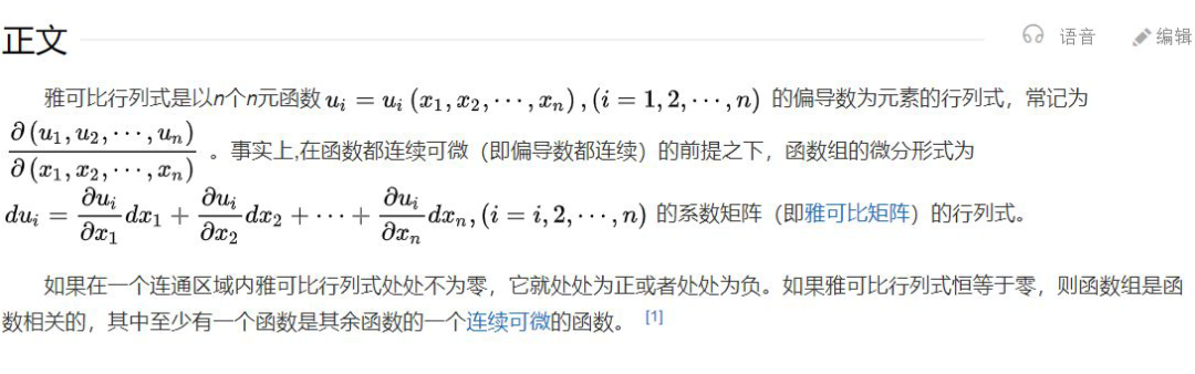
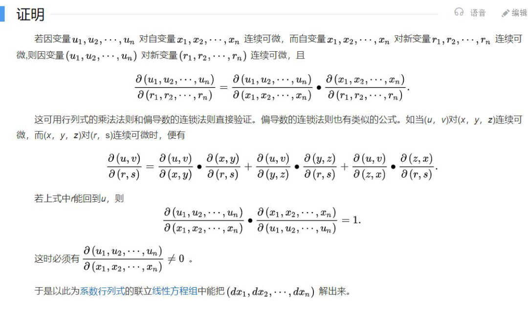
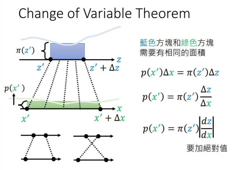
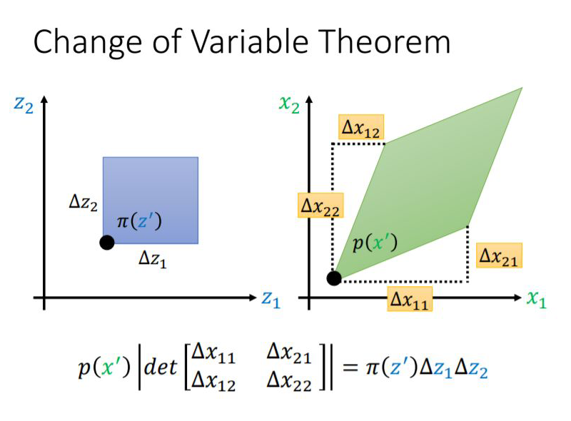
1.1 What is the Jacobian Determinant?
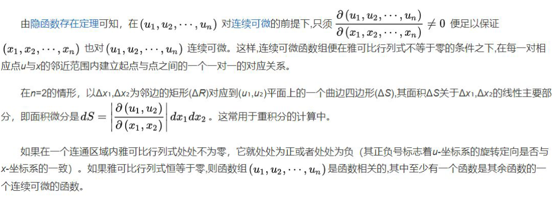
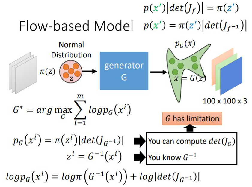
1.2 The Relationship Between Jacobian Determinant and Neural Networks
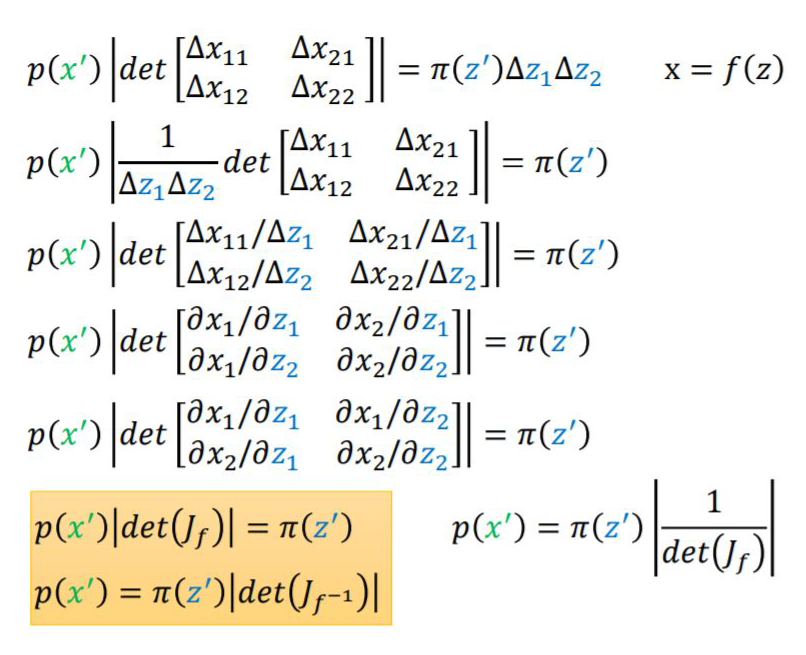
By the way, the loss function optimized for flow-based models is as follows:


1.3 Reversible Residual Network
Paper Title:
The Reversible Residual Network: Backpropagation Without Storing Activations
Paper Link:
https://arxiv.org/abs/1707.04585
Aidan N. Gomez and Mengye Ren from the University of Toronto proposed the reversible residual neural network, where the activation results of the current layer can be calculated from the results of the next layer. This means that if we know the final result of the network layer, we can backtrack to find the intermediate results of each previous layer. Therefore, we only need to store the parameters of the network and the results of the last layer, making the storage of activation results independent of the depth of the network, which will significantly reduce memory usage. Surprisingly, experimental results show that the performance of the reversible residual network does not significantly decline, and is comparable to previous experimental results of standard residual networks.
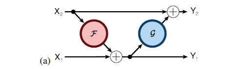


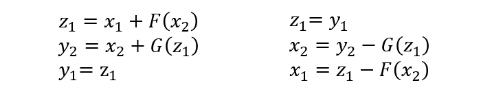
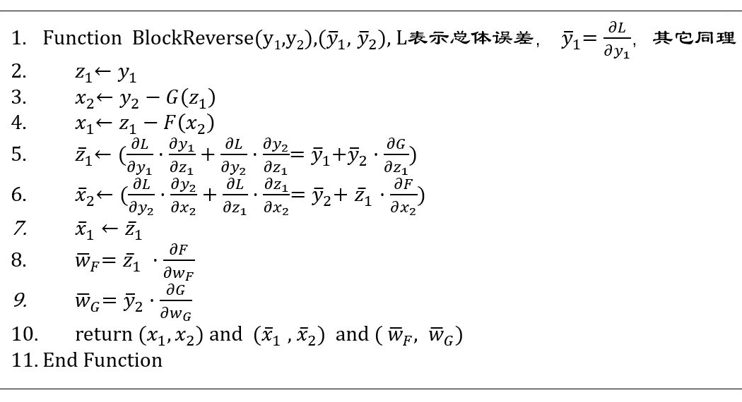
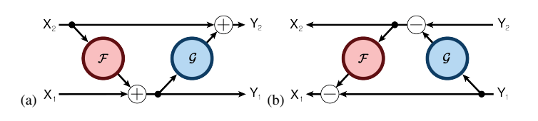
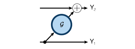
The encoding formula is as follows:


The decoding formula is as follows:


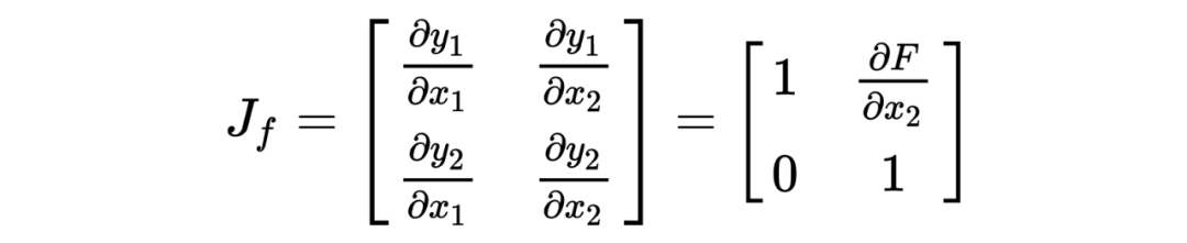
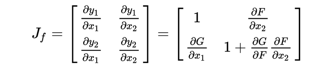
To compute the Jacobian matrix, we can write the encoding formula more intuitively as follows:


Its Jacobian matrix is:


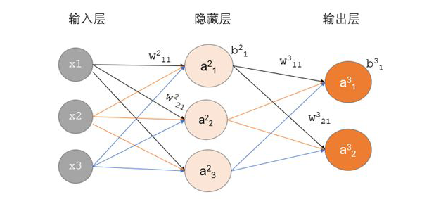
Backpropagation (BP) Algorithm
-
x1, x2, x3: Represents 3 input layer nodes. -
w: Represents the weight parameters from layer t-1 to layer t, j represents the j-th node in layer t, and i represents the i-th node in layer t-1. -
y: Represents the output result after activation of the i-th node in layer t. -
g(x): Represents the activation function.
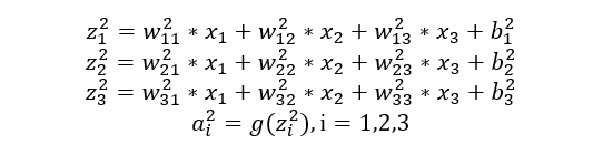
Forward Propagation Calculation Process:
-
Hidden Layer (the second layer of the network)
-
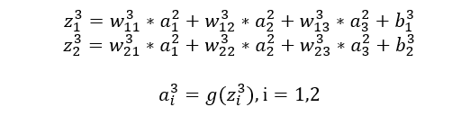
Output Layer (the last layer of the network)


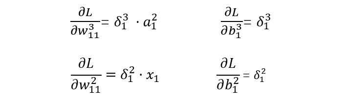
-
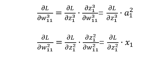
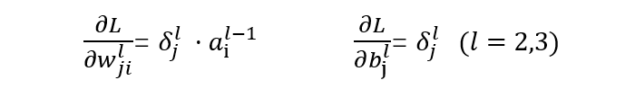
Output Layer

-
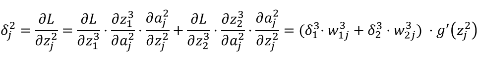
Hidden Layer

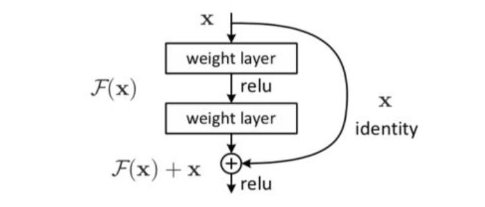
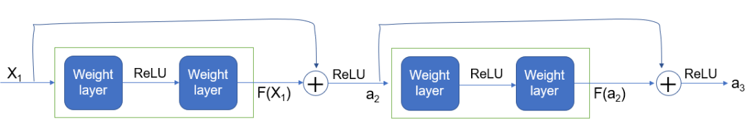
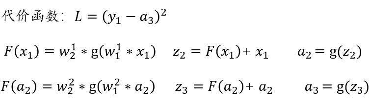
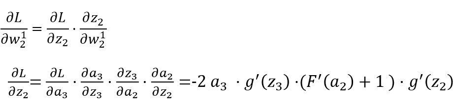
Residual Networks
-
Gradient vanishing problem;
-
Network degradation problem.

Editor: Huang Jiyan
Proofreader: Lin Yilin