

Source: DeepHub IMBA


This article is about 4300 words long and takes approximately 12 minutes to read.
This is an attempt to build a Gaussian Mixture Model (GMM) classifier using Pytorch.
We will build the Gaussian Mixture Model (GMM) from scratch. This will give us a basic understanding of the GMM, and this article will not cover the mathematics as we have done so in detail in previous articles.
This article will use the following libraries:
import torch import numpy as np import matplotlib.pyplot as plt import matplotlib.colors as mcolors
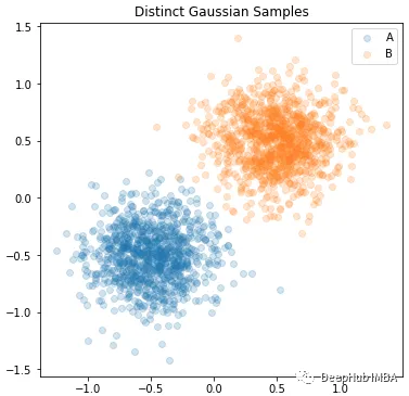
We will create 3 different Gaussian distributions (A, B, mix) in two dimensions, where mix should be a distribution made up of A and B.
First, the distributions of A and B…
 n_samples = 1000 A_means = torch.tensor( [-0.5, -0.5]) A_stdevs = torch.tensor( [0.25, 0.25]) B_means = torch.tensor( [0.5, 0.5]) B_stdevs = torch.tensor( [0.25, 0.25])
 A_dist = torch.distributions.Normal( A_means, A_stdevs) A_samp = A_dist.sample( [n_samples]) B_dist = torch.distributions.Normal( B_means, B_stdevs) B_samp = B_dist.sample( [n_samples])

 plt.figure( figsize=(6,6)) for name, sample in zip( ['A', 'B'], [A_samp, B_samp]):    plt.scatter( sample[:,0], sample[:, 1], alpha=0.2, label=name) plt.legend() plt.title( "Distinct Gaussian Samples") plt.show() plt.close()
To create a single mixed Gaussian distribution, we first vertically stack the means and standard deviations of A and B to generate new tensors, each with a shape of [2,2].
AB_means = torch.vstack( [ A_means, B_means]) AB_stdevs = torch.vstack( [ A_stdevs, B_stdevs])
The way Pytorch handles mixture distributions is by using three additional distributions: Independent, Categorical, and MixtureSameFamily on the original Normal distribution. Essentially, it creates a mixture based on the probability weights of the given Categorical distribution. Because our new means and standard sets have an additional axis, this axis is used as an independent axis to decide from which mean/standard set to draw values.
 AB_means = torch.vstack( [ A_means, B_means]) AB_stdevs = torch.vstack( [ A_stdevs, B_stdevs])
 AB_dist = torch.distributions.Independent( torch.distributions.Normal( AB_means, AB_stdevs), 1) mix_weight = torch.distributions.Categorical( torch.tensor( [1.0, 1.0])) mix_dist = torch.distributions.MixtureSameFamily( mix_weight, AB_dist)
Here, [1.0,1.0] indicates that the Categorical distribution should sample uniformly from each independent axis. To verify that it works, we will plot the values of each distribution…
A_samp = A_dist.sample( (500,)) B_samp = B_dist.sample( (500,)) mix_samp = mix_dist.sample( (500,)) plt.figure( figsize=(6,6)) for name, sample in zip( ['A', 'B', 'mix'], [A_samp, B_samp, mix_samp]): plt.scatter( sample[:,0], sample[:, 1], alpha=0.3, label=name) plt.legend() plt.title( "Original Samples with the new Mixed Distribution") plt.show() plt.close()

As can be seen, the new mix_samp distribution actually overlaps with our original two separate A and B distribution samples.
Model
Now we can start building our classifier.
First, we need to create an underlying GaussianMixModel, whose means, standard deviations, and classification weights can effectively be trained through the torch backpropagation and autograd system.
class GaussianMixModel( torch.nn.Module): def __init__(self, n_features, n_components=2): super().__init__() self.init_scale = np.sqrt( 6 / n_features) # What is the best scale to use? self.n_features = n_features self.n_components = n_components weights = torch.ones( n_components) means = torch.randn( n_components, n_features) * self.init_scale stdevs = torch.rand( n_components, n_features) * self.init_scale # # Our trainable Parameters self.blend_weight = torch.nn.Parameter(weights) self.means = torch.nn.Parameter(means) self.stdevs = torch.nn.Parameter(stdevs) def forward(self, x): blend_weight = torch.distributions.Categorical( torch.nn.functional.relu( self.blend_weight)) comp = torch.distributions.Independent(torch.distributions.Normal( self.means, torch.abs( self.stdevs)), 1) gmm = torch.distributions.MixtureSameFamily( blend_weight, comp) return -gmm.log_prob(x) def extra_repr(self) -> str: info = f" n_features={self.n_features}, n_components={self.n_components}, [init_scale={self.init_scale}]" return info @property def device(self): return next(self.parameters()).device
This model will return the negative log likelihood of each sample that falls within the domain of the mixture Gaussian distribution of the model.
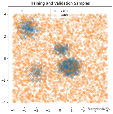
To train it, we need to provide samples from the mixture Gaussian distribution. To verify that it is effective, a batch of samples from a universal distribution will be provided to see how it can identify which samples might be similar to those in our training set.
train_means = torch.randn( (4,2)) train_stdevs = (torch.rand( (4,2)) + 1.0) * 0.25 train_weights = torch.rand( 4) ind_dists = torch.distributions.Independent( torch.distributions.Normal( train_means, train_stdevs), 1) mix_weight = torch.distributions.Categorical( train_weights) train_dist = torch.distributions.MixtureSameFamily( mix_weight, ind_dists) train_samp = train_dist.sample( [2000]) valid_samp = torch.rand( (4000, 2)) * 8 - 4.0 plt.figure( figsize=(6,6)) for name, sample in zip( ['train', 'valid'], [train_samp, valid_samp]): plt.scatter( sample[:,0], sample[:, 1], alpha=0.2, label=name) plt.legend() plt.title( "Training and Validation Samples") plt.show() plt.close()
The model only needs one hyperparameter n_components:
gmm = GaussianMixModel( n_features=2, n_components=4) gmm.to( 'cuda')
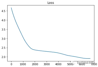
The training loop is also very simple:
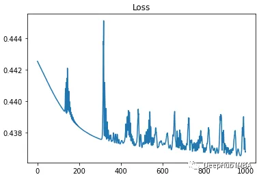
max_iter = 20000 features = train_samp.to( 'cuda') optim = torch.optim.Adam( gmm.parameters(), lr=5e-4) metrics = {'loss':[]} for i in range( max_iter): optim.zero_grad() loss = gmm( features) loss.mean().backward() optim.step() metrics[ 'loss'].append( loss.mean().item()) print( f"{i} ) {metrics[ 'loss'][-1]:0.5f}", end=f"{' '*20}\r") if metrics[ 'loss'][-1] < 0.1: print( "---- Close enough") break if len( metrics[ 'loss']) > 300 and np.std( metrics[ 'loss'][-300:]) < 0.0005: print( "---- Giving up") break print( f"Min Loss: {np.min( metrics[ 'loss']):0.5f}")
In this example, the loop stopped at a loss of 1.91043 in less than 7000 iterations.
If we now run the valid_samp samples through the model, we can convert the returned values into relative probabilities and redraw the validation data colored by predictions.
with torch.no_grad(): logits = gmm( valid_samp.to( 'cuda')) probs = torch.exp( -logits) plt.figure( figsize=(6,6)) for name, sample in zip( ['pred'], [valid_samp]): plt.scatter( sample[:,0], sample[:, 1], alpha=1.0, c=probs.cpu().numpy(), label=name) plt.legend() plt.title( "Testing Trained model on Validation") plt.show() plt.close()
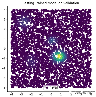
Our model has learned to recognize samples corresponding to the training distribution area. But we can also improve it.
Classification
With the above introduction, you should have a rough understanding of how to create a Gaussian Mixture Model and how to train it. The next step will use this information to build a composite (GMMClassifier) model that can learn to recognize different categories of mixed Gaussian distributions.
Here, a training set of overlapping Gaussian distributions is created, with 5 different classes, where each class itself is a mixture of Gaussian distributions.
This GMMClassifier will contain 5 different instances of GaussianMixModel. Each instance will attempt to learn a separate class from the training data. Each prediction will be combined into a set of classification logics, and the GMMClassifier will use these logics for predictions.
First, we need to make a small modification to the original GaussianMixModel and change the output from return -gmm.log_prob(x) to return gmm.log_prob(x). Since we are not directly trying to minimize this value in the training loop, it is used as the logits for our classification assignments.
The new model becomes…
class GaussianMixModel( torch.nn.Module): def __init__(self, n_features, n_components=2): super().__init__() self.init_scale = np.sqrt( 6 / n_features) # What is the best scale to use? self.n_features = n_features self.n_components = n_components weights = torch.ones( n_components) means = torch.randn( n_components, n_features) * self.init_scale stdevs = torch.rand( n_components, n_features) * self.init_scale # # Our trainable Parameters self.blend_weight = torch.nn.Parameter(weights) self.means = torch.nn.Parameter(means) self.stdevs = torch.nn.Parameter(stdevs) def forward(self, x): blend_weight = torch.distributions.Categorical( torch.nn.functional.relu( self.blend_weight)) comp = torch.distributions.Independent(torch.distributions.Normal( self.means, torch.abs( self.stdevs)), 1) gmm = torch.distributions.MixtureSameFamily( blend_weight, comp) return gmm.log_prob(x) def extra_repr(self) -> str: info = f" n_features={self.n_features}, n_components={self.n_components}, [init_scale={self.init_scale}]" return info @property def device(self): return next(self.parameters()).device
Our GMMClassifier code is as follows:
class GMMClassifier( torch.nn.Module): def __init__(self, n_features, n_classes, n_components=2): super().__init__() self.n_classes = n_classes self.n_features = n_features self.n_components = n_components if isinstance( n_components, list) else [n_components] * self.n_classes self.class_models = torch.nn.ModuleList( [ GaussianMixModel( n_features=self.n_features, n_components=self.n_components[i]) for i in range( self.n_classes)]) def forward(self, x, ret_logits=False): logits = torch.hstack( [ m(x).unsqueeze(1) for m in self.class_models]) if ret_logits: return logits return logits.argmax( dim=1) def extra_repr(self) -> str: info = f" n_features={self.n_features}, n_components={self.n_components}, [n_classes={self.n_classes}]" return info @property def device(self): return next(self.parameters()).device
When creating the model instance, a GaussianMixModel will be created for each class. Since each class may have a different number of components for its specific Gaussian mixture, we allow n_components to be a list of int values, which will be used when generating each underlying model. For example: n_components=[2,4,3,5,6] will pass the correct number of components to the class model. To simplify and set all underlying models to the same value, we can simply provide n_components=5, which will produce [5,5,5,5,5] when generating the model.
During training, logits need to be accessed, so the ret_logits parameter is provided in the forward() method. After training is complete, forward() can be called without parameters to return an int value for the predicted class (it only accepts the argmax of logits).
We will also create a set of 5 independent but overlapping Gaussian mixture distributions, each class having a random number of Gaussian components.
clusters = [0, 1, 2, 3, 4] features_group = {} n_samples = 2000 min_clusters = 2 max_clusters = 10 for c in clusters: features_group[ c] = [] n_clusters = torch.randint( min_clusters, max_clusters+1, (1,1)).item() print( f"Class: {c} Clusters: {n_clusters}") for i in range( n_clusters): mu = torch.randn( (1,2)) scale = torch.rand( (1,2)) * 0.35 + 0.05 distribution = torch.distributions.Normal( mu, scale) features_group[ c] += distribution.expand( (n_samples//n_clusters, 2)).sample() features_group[ c] = torch.vstack( features_group[ c]) features = torch.vstack( [features_group[ c] for c in clusters]).numpy() targets = torch.vstack( [torch.ones( (features_group[ c].size(0), 1)) * c for c in clusters]).view( -1).numpy() idxs = np.arange( features.shape[0]) valid_idxs = np.random.choice( idxs, 1000) train_idxs = [i for i in idxs if i not in valid_idxs] features_valid = torch.tensor( features[ valid_idxs]) targets_valid = torch.tensor( targets[ valid_idxs]) features = torch.tensor( features[ train_idxs]) targets = torch.tensor( targets[ train_idxs]) print( features.shape) plt.figure( figsize=(8,8)) for c in clusters: plt.scatter( features_group[c][:,0].numpy(), features_group[c][:,1].numpy(), alpha=0.2, label=c) plt.title( f"{n_samples} Samples Per Class, Multiple Clusters per Class") plt.legend()

By running the above code, we can know the number of n_components used by each class. In practice, it should be a hyperparameter search process, but here we already know, so we use it directly.
Class: 0 Clusters: 3 Class: 1 Clusters: 5 Class: 2 Clusters: 2 Class: 3 Clusters: 8 Class: 4 Clusters: 4
Then create the model:
gmmc = GMMClassifier( n_features=2, n_classes=5, n_components=[3, 5, 2, 8, 4]) gmmc.to( 'cuda')
The training loop also has some modifications, as we want to train the model with the classification loss provided by the logit predictions. Therefore, we need to provide targets during the supervised learning training process.
features = features.to( DEVICE) targets = targets.to( DEVICE) optim = torch.optim.Adam( gmmc.parameters(), lr=3e-2) loss_fn = torch.nn.CrossEntropyLoss() metrics = {'loss':[]} for i in range(4000): optim.zero_grad() logits = gmmc( features, ret_logits=True) loss = loss_fn( logits, targets.type( torch.long)) loss.backward() optim.step() metrics[ 'loss'].append( loss.item()) print( f"{i} ) {metrics[ 'loss'][-1]:0.5f}", end=f"{' '*20}\r") if metrics[ 'loss'][-1] < 0.1: print( "---- Close enough") break print( f"Mean Loss: {np.mean( metrics[ 'loss']):0.5f}")
Then classify the data from the validation data, which was generated when creating the training data, each sample is basically different values but from the appropriate class.
preds = gmmc( features_valid.to( 'cuda'))
Looking at the preds values, we can see that they are integers representing the predicted classes.
print( preds[0:10]) ____ tensor([2, 4, 2, 4, 2, 3, 4, 0, 2, 2], device='cuda:1')
Finally, by comparing these values with targets_valid, we can determine the accuracy of the model.
accuracy = (targets_valid == preds).sum() / targets_valid.size(0) * 100.0 print( f"Accuracy: {accuracy:0.2f}%") ____ Accuracy: 81.50%
We can also look at the accuracy of predictions for each class…
class_acc = {} for c in range(5): target_idxs = (targets_valid == c) class_acc[c] = (targets_valid[ target_idxs] == preds[ target_idxs]).sum() / targets_valid[ target_idxs].size(0) * 100.0 print( f"Class: {c} {class_acc[c]:0.2f}%") ---- Class: 0 98.54% Class: 1 69.06% Class: 2 86.12% Class: 3 70.05% Class: 4 84.09%
As can be seen, it performs better on classes with less overlap, which makes sense. And an average accuracy of 81.5% is quite good, considering all these different categories are overlapping. I believe there is still much room for improvement. If you have suggestions, or can point out mistakes I made, please leave a comment.
Author: Todd Shifflett
Editor: Huang Jiyan