Image Classification Techniques: KNN, SVM, BP Neural Networks, CNN, and Transfer Learning

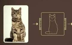
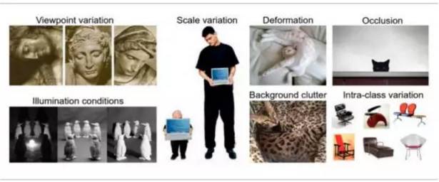
The image classification problem is the task of assigning labels to input images from a fixed set of categories. This is one of the core problems in computer vision. Although it seems simple, it has a variety of applications in real life.

Traditional Methods: Function Descriptions and Detection.

This method may be useful for some sample tasks, but the actual situation is much more complex.

Therefore, we will use machine learning to provide many examples for each category, and then develop learning algorithms to look at these examples and understand the visual appearance of each class, rather than trying to specify what each category of interest looks like directly in the code.

However, the image classification problem is a very complex task, which often borrows deep learning models such as Convolutional Neural Networks (CNN) to complete. But we also know that many algorithms we learn in class, such as KNN (K-Nearest Neighbors) and SVM (Support Vector Machine), perform very well on data mining problems, but they don’t always seem to be the best choice for image classification problems.

Therefore, we want to compare the performance of the algorithms we learned in class with CNN and transfer learning algorithms.

Goals

Our goals are:

1. To compare KNN, SVM, and BP neural networks with algorithms commonly used in industry for image classification problems, such as CNN and transfer learning.

2. To gain experience with deep learning.

3. To explore machine learning frameworks through Google’s TensorFlow.

Algorithms and Tools

The 5 methods we use in this project are KNN, SVM, BP neural networks, CNN, and transfer learning.

The entire project is mainly divided into 3 methods.

First Method: Use KNN, SVM, and BP neural networks, which are algorithms we learned in class, powerful and easy to implement. We mainly use sklearn to implement these algorithms.

Second Method: Although traditional multi-layer perceptron (MLP) models have been successfully applied to image recognition, they do not scale well to higher resolution images due to the complete connectivity between nodes being affected by the curse of dimensionality. So in this part, we use Google’s TensorFlow deep learning framework to build a CNN.

Third Method: Retrain the last layer of a pre-trained deep neural network (called Inception V3), also implemented by TensorFlow. Inception V3 was trained for the ImageNet Large Visual Recognition Challenge, with data collected starting in 2012. This is a standard task in computer vision, where the model attempts to classify the entire image into 1000 categories such as “zebra”, “spotted dog”, and “dishwasher”. To retrain this pre-trained network, we need to ensure that our own dataset has not been pre-trained.

How to Implement

First Method:

Preprocess the dataset and run KNN, SVM, and BP neural networks using sklearn.

First, we define two different preprocessing functions using the openCV package: the first is called image feature vector, which resizes the image and then flattens it into a row pixel list. The second is called extract color histogram, which uses cv2.normalize to extract a 3D color histogram from the HSV color space and then flattens the result.

Then, we construct several parameters to be parsed because we want to test the accuracy of this part not only for the entire dataset but also for subsets with different numbers of labels, and we will construct the dataset to be parsed into parameters in our program. Meanwhile, we also constructed the number of neighbors for the k-NN method as a parsing parameter.

After doing this, we begin to extract the features of each image in the dataset and put them into arrays. We use cv2.imread to read each image and split the labels by extracting strings from the image names. In our dataset, we use the same format for naming: “class label”.”image number”.jpg, so we can easily extract the class label of each image. Then we use the two functions defined earlier to extract two types of features and append them to the arrays rawImages and features, while the labels we extracted earlier are appended to the array labels.

The next step is to split the dataset using the function train_test_split imported from the sklearn package. The collections with suffixes RI and RL are the split results of rawImages and labels, while the other is the split result of features and labels. We use 85% of the dataset as the training set and 15% as the testing set.

Finally, we apply the KNN, SVM, and BP neural network functions to evaluate the data. For KNN, we use KNeighborsClassifier; for SVM, we use SVC; and for BP neural networks, we use MLPClassifier.

Second Method:

Build a CNN using TensorFlow. The purpose of TensorFlow is to allow you to build a computation graph (using any Python-like language) and then execute graph operations in C++, which is much more efficient than executing the same computations directly in Python.

TensorFlow can also automatically compute the gradients needed to optimize graph variables so that the model runs better. This is because the graph is a combination of simple mathematical expressions, and the chain rule of derivatives can be used to compute the gradients of the entire graph.

A TensorFlow graph consists of the following parts:

• Placeholder variables for inputting data into the graph.

• Variables to be optimized to make the convolutional network run better.

• The mathematical formulas of the convolutional network.

• Cost metrics that can be used to guide variable optimization.

• An optimization method to update variables.

The CNN architecture is formed by stacking different layers, which transforms input quantities into output quantities (e.g., class scores) through differentiable functions.

So in our implementation, the first layer saves the image, then we build 3 convolutional layers with 2×2 max pooling and Rectified Linear Units (ReLU).

The input is a four-dimensional tensor with the following dimensions:

• Number of images.

• Y-axis of each image.

• X-axis of each image.

• Channels of each image.

The output is another four-dimensional tensor with the following dimensions:

• Number of images, the same as input.

• Y-axis of each image. If a 2×2 pool is used, the height and width of the input image are divided by 2.

• X-axis of each image. Same as above.

• Channels produced by the convolutional filters.

Then we build 2 fully connected layers at the end of the network. The input is a 2D tensor with shape [num_images, num_inputs]. The output is a 2D tensor with shape [num_images, num_outputs].

However, to connect the convolutional layers and fully connected layers, we need a flattening layer to reduce the 4D tensor to 2D so that it can be used as input for the fully connected layers.

The last part of the CNN is always a softmax layer, which normalizes the output from the fully connected layer so that each element is constrained between 0 and 1, and all elements sum to 1.

To optimize the training results, we need a cost metric and minimize it at each iteration. The cost function we use here is cross-entropy (called from tf.nn.softmax_cross_entropy_with_logits()), and we take the average of cross-entropy for all image classifications. The optimization method is tf.train.AdamOptimizer(), which is a higher-level form of Gradient Descent. This is a tuned learning rate.

Third Method:

Retrain the Inception V3 object recognition model, which has millions of parameters and may take weeks to train fully. Transfer learning is a technique that can quickly accomplish this by adopting a pre-trained model for a set of categories (like ImageNet) and training from the existing weights of new categories. Although it does not perform as well as a fully trained run, it is very effective for many applications and can run on a laptop, taking only thirty minutes without a GPU. For the implementation of this part, we can follow the instructions below:

https://www.tensorflow.org/tutorials/image_retraining

First, we need to obtain the pre-trained model, remove the old top layer, and train a new model on our dataset. In a raw ImageNet class without cat breeds, we need to train the entire network. The magic of transfer learning is that the lower layers trained to distinguish certain objects can be reused for many recognition tasks without any changes. Then we analyze all the images on disk and calculate the bottleneck values for each image. Click here for details about bottlenecks (https://www.tensorflow.org/tutorials/image_retraining). Each image is reused multiple times during training, so calculating each bottleneck value takes a lot of time, so caching these bottleneck values can speed things up and avoid recalculating.

The script will run 4000 training steps. Each step randomly selects ten images from the training set, discovers their bottlenecks from the cache, and feeds them into the last layer for predictions. Then these predictions are compared with the actual labels, updating the weights of the final layer through the backpropagation process.

Start Experimenting

Dataset

Oxford IIIT Pet Dataset (http://www.robots.ox.ac.uk/~vgg/data/pets/)

Contains 25 breeds of dogs and 12 breeds of cats. Each breed has 200 images.

We only used 10 cat breeds in the project.

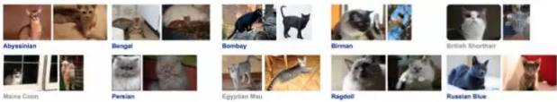
The types we used here are [‘Sphynx’ (Canadian Hairless Cat, also known as Sphinx Cat), ‘Siamese’ (Siamese Cat), ‘Ragdoll’ (Ragdoll Cat), ‘Persian’ (Persian Cat), ‘Maine-Coon’ (Maine Coon), ‘British-shorthair’ (British Shorthair), ‘Bombay’ (Bombay Cat), ‘Birman’ (Burmese Cat), ‘Bengal’ (Bengal Cat)].

So we have a total of 2000 images in the dataset, each with different sizes. However, I can resize them to a fixed size, such as 64 x 64 or 128 x 128.

Preprocessing

In this project, we mainly use OpenCV for processing image data, such as reading images into arrays and resizing them to the required size.

A common method to improve image training results is to randomly deform, crop, or enhance training inputs, which has the advantage of effectively expanding the size of the training data by all possible variations of the same image, and tends to help the network learn to cope with all the distortion problems that will occur in the real use of the classifier.

For details, see the link: https://github.com/aleju/imgaug

Evaluation

First Method:

First part: Preprocess the dataset and apply KNN, SVM, and BP neural networks using sklearn.

There are many parameters to adjust in the program: in the image_to_feature_vector function, we set the size to 128×128, and we previously tried sizes like 8×8, 64×64, 256×256. Thus we found that the larger the image size, the better the accuracy. However, larger image sizes also increase execution time and memory consumption. So we finally decided on an image size of 128×128, as it is not too large but can still ensure accuracy.

In the extract_color_histogram function, we set the number of bins for each channel to be 32, 32, 32. Like the previous function, we also tried 8, 8, 8 and 64, 64, 64, and higher numbers can produce better results, but also come with increased execution time. So we think 32, 32, 32 is the most suitable.

As for the dataset, we tried three datasets. The first is a subset with 400 images and 2 labels. The second is a subset with 1000 images and 5 labels. The last one is the entire dataset with 1997 images and 10 labels. And we parsed different datasets into parameters in the program.

In KNeighborsClassifier, we only changed the number of neighbors and stored the results as the best K for each dataset. Then we set all other parameters to default values.

In MLPClassifier, we set a hidden layer with 50 neurons. We tested multiple hidden layers, but the final results did not seem to change much. The maximum iteration time was set to 1000, with a tolerance of 1e-4 to ensure convergence. We set the L2 penalty parameter α to default, random state to 1, solver to “sgd”, and learning rate to 0.1.

In SVC, the maximum iteration time is 1000, and the class weight value is “balanced”.

The runtime of our program is not very long, taking about 3 to 5 minutes from the 2-label dataset to the 10-label dataset.

Second Method:

Build a CNN using TensorFlow.

Calculating the gradients of the model takes a long time since this model uses the entirety of a large dataset. Therefore, we only use a small number of images in each iteration of the optimizer. The batch size is typically 32 or 64. The dataset is divided into a training set containing 1600 images, a validation set containing 400 images, and a test set containing 300 images.

There are many parameters that can be adjusted.

First is the learning rate. As long as it is small enough to converge and large enough not to slow down the program too much, a good learning rate is relatively easy to find. We chose 1×10 ^ -4.

The second is the size of the images we provide to the network. We tried 64 * 64 and 128 * 128. It turns out that the larger the image, the higher the accuracy we get, but at the cost of increased runtime.

Then there are the layers and their shapes. But in reality, there are too many parameters to adjust, so finding the optimal values for these parameters is a very challenging task.

According to many online resources, we have learned that the choice of parameters for building the network almost entirely depends on experience.

Initially, we tried to build a relatively complex network with parameters as follows:

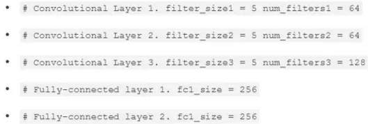
We used 3 convolutional layers and 2 fully connected layers, which are relatively complex.

However, the result was — overfitting. Only after a thousand iterations did our program achieve 100% training accuracy, while only 30% test accuracy. Initially, I was confused as to why we got an overfitting result, and I tried to randomly adjust parameters, but the results never improved. A few days later, I happened to see an article discussing a deep learning project conducted by Chinese researchers (https://medium.com/@blaisea/physiognomys-new-clothes-f2d4b59fdd6a). They pointed out that the research they conducted had problems. “A technical issue is that wanting to train and test a CNN like AlexNet without overfitting is not achievable with less than 2000 examples.” So at that moment, I realized that first, our dataset is actually small, and second, our network is too complex.

Remember, our dataset contains exactly 2000 images.

Then I tried to reduce the number of layers and the size of the kernels. I tried many parameters, and the following image shows the final structure we used.

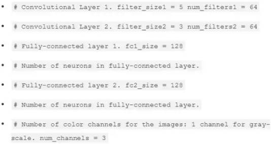
We only used 2 small-sized convolutional layers and 2 fully connected layers. The results were not very ideal; even after 4000 iterations, the results were still overfitting, but the test results improved by 10% compared to before.

We are still looking for a way to handle it, but the obvious reason is that our dataset is insufficient, and we do not have enough time for better improvements.

The final result is that after 5000 iterations, we reached about 43% accuracy, while the runtime exceeded half an hour.

PS: In fact, due to this result, we felt a bit uneasy. So we found another standard dataset — CIFAR-10 (https://www.cs.toronto.edu/~kriz/cifar.html).

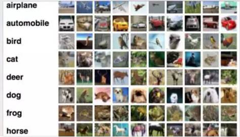
The CIFAR-10 dataset consists of 60,000 32×32 color images in 10 categories, with 6,000 images per category. It contains 50,000 training images and 10,000 test images.

We used the same network constructed above, and after 10 hours of training, we achieved 78% accuracy on the test set.

Third Method:

Retrain Inception V3. Similarly, we randomly select several images for training and choose another batch of images for validation.

There are many parameters that can be adjusted.

First is the training steps, the default is 4000. If we can get a reasonable result earlier, we try more or try a smaller one.

The learning rate controls the size of updates to the last layer during training. Intuitively, if it is smaller, learning will take longer but can ultimately help improve overall accuracy. **train batch** size controls the number of images checked in one training step, and since the learning rate is applied to each batch, if you want to have larger batches to achieve the same overall effect, we will need to reduce their number.

Since deep learning tasks are heavy, runtimes are usually relatively long, so we do not want to find out after several hours of training that our model is actually very poor. Therefore, we often check the accuracy of validation. This way, we can also avoid overfitting. By splitting, we can place 80% of the images into the main training set, keeping 10% for validation during training, running frequently, and then using the final 10% of the images as the test set to predict the classifier’s performance in the real world.

Results

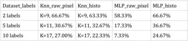
First Method: Preprocess the dataset and run KNN, SVM, and BP neural networks using sklearn.

The results are shown in the figure below. Since the results for SVM were very poor, even lower than random guessing, we did not provide its running results.

From the results, we can see:

In k-NN, the raw pixel accuracy and histogram accuracy are relatively the same. In the subset containing 5 labels, the histogram accuracy is slightly higher than the raw pixel accuracy, but among all raw pixels, the raw pixel shows better results.

In the neural network MLP classifier, the raw pixel accuracy is far lower than the histogram accuracy. For the entire dataset (containing 10 labels), the raw pixel accuracy is even lower than random guessing.

Both of these sklearn methods did not provide very good performance, with an accuracy of only about 24% for correctly identifying categories in the entire dataset (containing 10 labels). These results indicate that using sklearn methods for image recognition is not effective. They do not perform well in classifying complex images with multiple categories. However, compared to random guessing, they did make some improvements, but it is still far from enough.

Based on this result, we found that to improve accuracy, some deep learning methods must be adopted.

Second Method: Using TensorFlow to build the CNN as described above, we could not achieve good results due to overfitting.

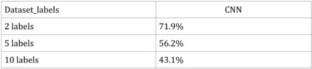
The training usually takes about half an hour, but due to the results being overfitted, we consider this runtime unimportant. Compared to Method 1, we can see that although the results of the CNN are overfitted, we still get better results than Method 1.

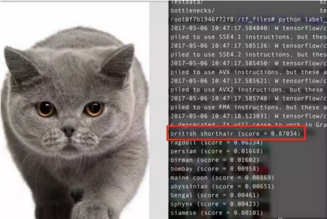
Third Method: Retraining Inception V3.

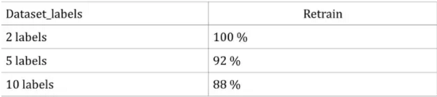
The entire training process took no more than 10 minutes, and we can achieve very good results. Based on this, we can actually see the tremendous power of deep learning and transfer learning.

Demonstration:

Goals

Based on the above comparisons, we can draw the following conclusions:

KNN, SVM, and BP neural networks cannot perform well on specific tasks such as image classification.

Although we obtained overfitting results in the CNN part, they are still much better than the other methods learned in class for handling image classification problems.

Transfer learning is very efficient for image classification problems. It can accurately and quickly complete training in a short time without a GPU. Even if you have a small dataset, it can effectively prevent overfitting.

We learned some very important experiences in image classification tasks. Such tasks are completely different from the other tasks we did in class. The dataset is relatively large and not sparse, and the network is complex, so if you do not use a GPU, the runtime will be quite long.

Crop or resize images to make them smaller.

Randomly select a small batch for training in each iteration.

Randomly select a small batch for validation during training and frequently report validation scores.

Try using image augmentation to transform a set of input images into a new, larger set of slightly altered images.

For image classification tasks, we need a larger dataset than 200 x 10; the CIFAR10 dataset contains 60,000 images.

More complex networks require more datasets for training.

Be aware of overfitting.

Click on the end of the article “Read Original” to view the open-source code on GitHub.

To ensure the quality of the publication and establish a good reputation, Data Dispatch has set up a “Typo Fund”, encouraging readers to actively correct errors.

If you find any errors while reading the article, please leave a comment at the end of the article or feedback to the background. After confirmation by the editor, Data Dispatch will send a 8.8 yuan red envelope to the reporting reader.

Thank you for your continued attention and support, and we hope you can supervise Data Dispatch to produce higher quality content.