Hands-On Guide: Deep Learning with PyTorch (Code Included)

Original Title:

An Introduction to PyTorch – A Simple yet Powerful Deep Learning Library

Author: FAIZAN SHAIKH

Translator: He Zhonghua

This article is about 3600 words, recommended reading time is 15 minutes.This article will guide you step by step through PyTorch with practical examples.

Introduction

Every once in a while, a Python library emerges that has the potential to change the landscape of deep learning, and PyTorch is one of them.

Over the past few weeks, I have been immersed in PyTorch, attracted by its ease of use. Among various deep learning libraries I have used, PyTorch is the most flexible and user-friendly so far.

In this article, we will explore PyTorch in a more practical way, covering the basics and case studies. We will also compare neural networks built from scratch using NumPy and PyTorch to see their similarities in specific implementations.

Let’s get started!

Note: This article assumes you have a basic understanding of deep learning. If you want a quick overview, please read this article here.

Table of Contents

• Overview of PyTorch

• Technical Deep Dive

• Numpy VS. PyTorch in Building Neural Networks

• Comparison with Other Deep Learning Libraries

• Case Study – Solving Image Recognition Problems with PyTorch

Overview of PyTorch

The creators of PyTorch say they adhere to an imperative programming philosophy. This means we can run computations immediately. This aligns perfectly with Python’s programming methodology, as we don’t have to wait until the entire code is written to know if it runs. We can easily run parts of the code and check them in real-time. For someone like me, who debugs neural networks, this is a blessing.

PyTorch is a Python-based library designed to provide a flexible deep learning development platform.

PyTorch’s workflow is as close as possible to Python’s scientific computing library—NumPy.

You may ask, why use PyTorch to build deep learning models? Here are three reasons:

• User-Friendly API: As simple and easy to use as Python;

• Supports Python: As mentioned, PyTorch integrates smoothly with the Python data science stack. It is so similar to NumPy that you might not even notice the differences;

• Dynamic Computation Graph: PyTorch does not provide a predefined graph with specific functions, but instead provides us with a framework to build computation graphs, which we can even modify at runtime. This is useful in situations where we are not sure how much memory we need when creating a neural network.

There are other benefits to using PyTorch, such as support for multiple GPUs, custom data loaders, and simplified preprocessors.

Since its release in early January 2016, many researchers have incorporated it into their toolbox because it is easy to build novel and even very complex graphs. That said, it will take time for PyTorch to be widely accepted by most data science practitioners, as it is both a new thing and still “under construction”.

Technical Deep Dive

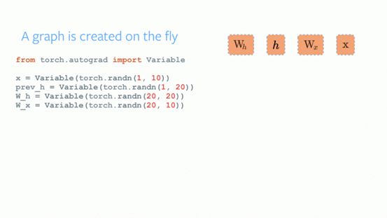
Before diving into the details, let’s understand the workflow of PyTorch.

PyTorch employs an imperative programming paradigm. This means that every line of code needed to build the graph defines a component of that graph. Even before the graph is fully constructed, we can independently perform computations on these components. This is known as the “define-by-run” method.

Source: http://pytorch.org/about/

Installing PyTorch is very simple. You can follow the steps mentioned in the official documentation based on your system. For example, here are the commands used based on my options:

conda install pytorch torchvision cuda91 -c pytorch

The main elements we should understand before we start using PyTorch are:

• PyTorch Tensors

• Mathematical Operations

• Autograd Module

• Optim Module

• nn Module

Next, we will detail each part.

1. PyTorch Tensors

A tensor is a multi-dimensional array. Tensors in PyTorch are similar to ndarrays in NumPy, and in addition, tensors in PyTorch can also be used on the GPU. PyTorch supports various types of tensors.

You can define a simple one-dimensional matrix as follows:

# import pytorch
import torch

# define a tensor
torch.FloatTensor([2])

2
[torch.FloatTensor of size 1]

2. Mathematical Operations

Like NumPy, it is essential for scientific computing libraries to implement mathematical functions effectively. PyTorch provides a similar interface, allowing you to use over 200 mathematical operations.

Here is a simple example of an addition operation:

a = torch.FloatTensor([2])
b = torch.FloatTensor([3])
a + b

5
[torch.FloatTensor of size 1]

Doesn’t this look like a typical Python method? We can also perform various matrix operations on defined PyTorch tensors. For example, we can transpose a two-dimensional matrix:

matrix = torch.randn(3, 3)
matrix

-1.3531 -0.5394  0.8934
 1.7457 -0.6291 -0.0484
-1.3502 -0.6439 -1.5652
[torch.FloatTensor of size 3x3]

matrix.t()

-1.3531  1.7457  -1.3502
-0.5394 -0.6291  -0.6439
 0.8934  -0.0484  -1.5652
[torch.FloatTensor of size 3x3]

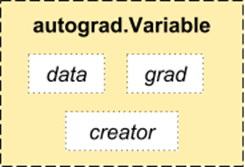
3. Autograd Module

PyTorch uses a technique called automatic differentiation. This means we have a recorder that logs the operations we have performed, and then it plays back to compute our gradients. This technique is particularly useful when building neural networks, as we compute the derivatives of parameters during forward propagation, which can reduce computation time for each epoch.

Source: http://pytorch.org/about/

from torch.autograd import Variable

x = Variable(train_x)
y = Variable(train_y, requires_grad=False)

4. Optim Module

Torch.optim is a module that implements various optimization algorithms for building neural networks. Most commonly used methods are supported, so we don’t have to build them from scratch (unless you want to!).

Here is a piece of code using the Adam optimizer:

optimizer = torch.optim.Adam(model.parameters(), lr=learning_rate)

5. nn Module

PyTorch’s autograd can easily define computation graphs and compute gradients, but the raw autograd may be a bit too low-level for defining complex neural networks. This is where the nn module comes in handy.

The nn package defines a set of modules that we can think of as a neural network layer that produces output from input and may have some trainable weights.

You can think of the nn module as PyTorch’s Keras!

import torch

# define model
model = torch.nn.Sequential(
 torch.nn.Linear(input_num_units, hidden_num_units),
 torch.nn.ReLU(),
 torch.nn.Linear(hidden_num_units, output_num_units),
)

loss_fn = torch.nn.CrossEntropyLoss()

Now that you know the basic components of PyTorch, you can easily build your own neural networks from scratch. If you want to know how to do it specifically, keep reading.

Numpy VS. PyTorch in Building Neural Networks

I previously mentioned that PyTorch and NumPy are very similar, so let’s see why. In this section, we will see how a simple neural network for solving a binary classification problem is implemented. You can get an in-depth explanation here.

## Neural network in numpy

import numpy as np

#Input array
X=np.array([[1,0,1,0],[1,0,1,1],[0,1,0,1]])

#Output
y=np.array([[1],[1],[0]])

#Sigmoid Function
def sigmoid (x):
 return 1/(1 + np.exp(-x))

#Derivative of Sigmoid Function
def derivatives_sigmoid(x):
 return x * (1 - x)

#Variable initialization
epoch=5000 #Setting training iterations
lr=0.1 #Setting learning rate
inputlayer_neurons = X.shape[1] #number of features in data set
hiddenlayer_neurons = 3 #number of hidden layers neurons
output_neurons = 1 #number of neurons at output layer

#weight and bias initialization
wh=np.random.uniform(size=(inputlayer_neurons,hiddenlayer_neurons))
bh=np.random.uniform(size=(1,hiddenlayer_neurons))
wout=np.random.uniform(size=(hiddenlayer_neurons,output_neurons))
bout=np.random.uniform(size=(1,output_neurons))

for i in range(epoch):
  #Forward Propogation
  hidden_layer_input1=np.dot(X,wh)
  hidden_layer_input=hidden_layer_input1 + bh
  hiddenlayer_activations = sigmoid(hidden_layer_input)
  output_layer_input1=np.dot(hiddenlayer_activations,wout)
  output_layer_input= output_layer_input1+ bout
  output = sigmoid(output_layer_input)

  #Backpropagation
  E = y-output
  slope_output_layer = derivatives_sigmoid(output)
  slope_hidden_layer = derivatives_sigmoid(hiddenlayer_activations)
  d_output = E * slope_output_layer
  Error_at_hidden_layer = d_output.dot(wout.T)
  d_hiddenlayer = Error_at_hidden_layer * slope_hidden_layer
  wout += hiddenlayer_activations.T.dot(d_output) *lr
  bout += np.sum(d_output, axis=0,keepdims=True) *lr
  wh += X.T.dot(d_hiddenlayer) *lr
  bh += np.sum(d_hiddenlayer, axis=0,keepdims=True) *lr

print('actual :
', y, '
')
print('predicted :
', output)

Now, try to discover the super simple implementation of PyTorch compared to the previous one (the differences are highlighted in bold in the code below).

## neural network in pytorch
import torch

#Input array
X = torch.Tensor([[1,0,1,0],[1,0,1,1],[0,1,0,1]])
#Output
y = torch.Tensor([[1],[1],[0]])
#Sigmoid Function
def sigmoid (x):
  return 1/(1 + torch.exp(-x))
#Derivative of Sigmoid Function
def derivatives_sigmoid(x):
  return x * (1 - x)
#Variable initialization
epoch=5000 #Setting training iterations
lr=0.1 #Setting learning rate
inputlayer_neurons = X.shape[1] #number of features in data set
hiddenlayer_neurons = 3 #number of hidden layers neurons
output_neurons = 1 #number of neurons at output layer
#weight and bias initialization
wh=torch.randn(inputlayer_neurons, hiddenlayer_neurons).type(torch.FloatTensor)
bh=torch.randn(1, hiddenlayer_neurons).type(torch.FloatTensor)
wout=torch.randn(hiddenlayer_neurons, output_neurons)
bout=torch.randn(1, output_neurons)

for i in range(epoch):
  #Forward Propogation
  hidden_layer_input1 = torch.mm(X, wh)
  hidden_layer_input = hidden_layer_input1 + bh
  hiddenlayer_activations = sigmoid(hidden_layer_input)
  output_layer_input1 = torch.mm(hiddenlayer_activations, wout)
  output_layer_input = output_layer_input1 + bout
  output = sigmoid(output_layer_input1)
  #Backpropagation
  E = y-output
  slope_output_layer = derivatives_sigmoid(output)
  slope_hidden_layer = derivatives_sigmoid(hiddenlayer_activations)
  d_output = E * slope_output_layer
  Error_at_hidden_layer = torch.mm(d_output, wout.t())
  d_hiddenlayer = Error_at_hidden_layer * slope_hidden_layer
  wout += torch.mm(hidden_layer_activations.t(), d_output) *lr
  bout += d_output.sum() *lr
  wh += torch.mm(X.t(), d_hiddenlayer) *lr
  bh += d_output.sum() *lr
print('actual :
', y, '
')
print('predicted :
', output)

• Comparison with Other Deep Learning Libraries

In a benchmark script, comparing the median time of the lowest epoch, PyTorch outperformed all other major deep learning libraries in training a Long Short Term Memory (LSTM) network, as shown in the figure below:

The APIs for data loading are well designed in PyTorch. Interfaces are specified in datasets, samplers, and data loaders.

When comparing data loading tools in TensorFlow (readers, queues, etc.), I found that the data loading module in PyTorch is very easy to use. Additionally, PyTorch integrates seamlessly when we try to build neural networks, so we don’t have to rely on third-party high-level libraries like Keras (which depends on TensorFlow or Theano).

On the other hand, I do not recommend using PyTorch for deployment. PyTorch is still in development. As the PyTorch developers say: “What we see is users first create a PyTorch model, and when they are ready to deploy the model to production, they simply convert it to a Caffe 2 model and then publish it to mobile platforms or other platforms.”

Case Study: Solving Image Recognition Problems with PyTorch

To get familiar with PyTorch, we will tackle a deep learning practical problem from Analytics Vidhya – recognizing digits. Let’s take a look at our problem statement:

Our problem is an image recognition problem, identifying digits from a given 28×28 pixel image. We have part of the images for training and the rest for testing our model.

First, download the training and testing files. The dataset contains a compressed file of all images, and both train.csv and test.csv have the names of the respective training and testing images. No other features are provided in the dataset, just the raw images in ‘.png’ format.

Let’s get started:

Step 0: Preparation

1. Import all necessary libraries:

# import modules
%pylab inline
import os
import numpy as np
import pandas as pd
from scipy.misc import imread
from sklearn.metrics import accuracy_score

2. Set a seed value so we can control the randomness of the model

# To stop potential randomness
seed = 128
rng = np.random.RandomState(seed)

3. The first step is to set the directory path to save safely!

root_dir = os.path.abspath('.')
data_dir = os.path.join(root_dir, 'data')

# check for existence
os.path.exists(root_dir), os.path.exists(data_dir)

Step 1: Data Loading and Preprocessing

1. Now we will read the dataset. They are in .csv format and have corresponding labels in their filenames.

# load dataset
train = pd.read_csv(os.path.join(data_dir, 'Train', 'train.csv'))
test = pd.read_csv(os.path.join(data_dir, 'Test.csv'))

sample_submission = pd.read_csv(os.path.join(data_dir, 'Sample_Submission.csv'))

train.head()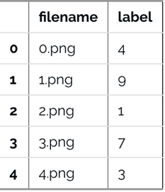

2. Let’s take a look at what the data looks like, read the image, and display it.

# print an image
img_name = rng.choice(train.filename)
filepath = os.path.join(data_dir, 'Train', 'Images', 'train', img_name)

img = imread(filepath, flatten=True)

pylab.imshow(img, cmap='gray')
pylab.axis('off')
pylab.show()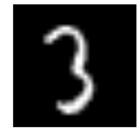

3. For easier data manipulation, we will store all images as numpy arrays.

# load images to create train and test set
temp = []
for img_name in train.filename:
  image_path = os.path.join(data_dir, 'Train', 'Images', 'train', img_name)
  img = imread(image_path, flatten=True)
  img = img.astype('float32')
  temp.append(img)
train_x = np.stack(temp)

train_x /= 255.0
train_x = train_x.reshape(-1, 784).astype('float32')

temp = []
for img_name in test.filename:
  image_path = os.path.join(data_dir, 'Train', 'Images', 'test', img_name)
  img = imread(image_path, flatten=True)
  img = img.astype('float32')
  temp.append(img)
test_x = np.stack(temp)

test_x /= 255.0
test_x = test_x.reshape(-1, 784).astype('float32')

train_y = train.label.values

4. Since this is a typical ML problem, to test the correct functionality of our model, we create a validation set. We split the training set and validation set in a 70:30 ratio.

# create validation set
split_size = int(train_x.shape[0]*0.7)
train_x, val_x = train_x[:split_size], train_x[split_size:]
train_y, val_y = train_y[:split_size], train_y[split_size:]

Step 2: Build the Model

5. Now comes the main part, defining our neural network architecture. We define a 3-layer neural network consisting of input, hidden, and output layers. The number of neurons in the input and output layers is fixed, as the input is our 28×28 image, and the output is a 10×1 vector representing classes. We use 50 neurons in the hidden layer. Here, we use Adam as the optimization algorithm, which is an effective variant of gradient descent.

import torch
from torch.autograd import Variable
# number of neurons in each layer
input_num_units = 28*28
hidden_num_units = 500
output_num_units = 10
# set remaining variables
epochs = 5
batch_size = 128
learning_rate = 0.001

6. It’s time to train the model

# define model
model = torch.nn.Sequential(
  torch.nn.Linear(input_num_units, hidden_num_units),
  torch.nn.ReLU(),
  torch.nn.Linear(hidden_num_units, output_num_units),
)

loss_fn = torch.nn.CrossEntropyLoss()

# define optimization algorithm
optimizer = torch.optim.Adam(model.parameters(), lr=learning_rate)

## helper functions
# preprocess a batch of dataset
def preproc(unclean_batch_x):
  """Convert values to range 0-1"""
  temp_batch = unclean_batch_x / unclean_batch_x.max()
  return temp_batch
# create a batch
def batch_creator(batch_size):
  dataset_name = 'train'
  dataset_length = train_x.shape[0]
  batch_mask = rng.choice(dataset_length, batch_size)
  batch_x = eval(dataset_name + '_x')[batch_mask]
  batch_x = preproc(batch_x)
  if dataset_name == 'train':
    batch_y = eval(dataset_name).ix[batch_mask, 'label'].values
  return batch_x, batch_y

# train network
total_batch = int(train.shape[0]/batch_size)

for epoch in range(epochs):
  avg_cost = 0
  for i in range(total_batch):
    # create batch
    batch_x, batch_y = batch_creator(batch_size)
    # pass that batch for training
    x, y = Variable(torch.from_numpy(batch_x)), Variable(torch.from_numpy(batch_y), requires_grad=False)
    pred = model(x)
    # get loss
    loss = loss_fn(pred, y)
    # perform backpropagation
    loss.backward()
    optimizer.step()
    avg_cost += loss.data[0]/total_batch
  print(epoch, avg_cost)

# get training accuracy
x, y = Variable(torch.from_numpy(preproc(train_x))), Variable(torch.from_numpy(train_y), requires_grad=False)
pred = model(x)

final_pred = np.argmax(pred.data.numpy(), axis=1)

accuracy_score(train_y, final_pred)

# get validation accuracy
x, y = Variable(torch.from_numpy(preproc(val_x))), Variable(torch.from_numpy(val_y), requires_grad=False)
pred = model(x)

final_pred = np.argmax(pred.data.numpy(), axis=1)

accuracy_score(val_y, final_pred)

The training score is:

0.8779008746355685

And the validation score is:

0.867482993197279

This is quite an impressive score, especially since we trained a very simple neural network for just 5 epochs.

Conclusion

I hope this article has shown you how PyTorch can change the way we build deep learning models. In this article, we have only scratched the surface. For a deeper dive, you can read the documentation and tutorials on the official PyTorch page.

In the upcoming articles, I will use PyTorch for audio analysis, and we will try to build deep learning models for speech processing. Stay tuned!

Have you used PyTorch to build applications or in any data science projects? Please let me know in the comments below.

Original link:

https://www.analyticsvidhya.com/blog/2018/02/pytorch-tutorial/

Translator’s Profile

He Zhonghua, a master’s student in software engineering in Germany. Due to an interest in machine learning, I chose to improve traditional k-means using genetic algorithm ideas for my master’s thesis. Currently, I am practicing big data-related work in Hangzhou. Joining Datapi THU, I hope to contribute a little to my IT peers and make many like-minded friends.

Translation Team Recruitment Information

Job Content: Accurately translate selected cutting-edge foreign articles into fluent Chinese. If you are a data science/statistics/computer major studying abroad, or working overseas in related fields, or confident in your foreign language skills, the Datapi translation team welcomes you to join!

What you will gain: Improve your understanding of cutting-edge data science, enhance your awareness of foreign news sources, and overseas friends can stay connected with domestic technology application developments. The academic and research background of the Datapi team provides good development opportunities for volunteers.

Other Benefits: Collaborate and communicate with data science professionals from well-known companies, students from prestigious universities such as Peking University and Tsinghua University, and other top schools abroad.

Click at the end of the article “Read the Original” to join the Datapi team~

Reprint Notice

For reprints, please indicate the author and source prominently at the beginning (Reprinted from: Datapi THU ID: DatapiTHU), and place the Datapi QR code at the end of the article. For articles with original identification, please send [Article Name – Waiting for Authorization Public Account Name and ID] to the contact email to apply for whitelist authorization and edit according to requirements.

After publication, please feedback the link to the contact email (see below). Unauthorized reprints and adaptations will be legally pursued.

Click “Read the Original” to embrace the organization