
MLNLP(Machine Learning Algorithms and Natural Language Processing) is one of the largest natural language processing communities in China and abroad, gathering over 500,000 subscribers, covering domestic and international NLP master’s and doctoral students, university teachers, and corporate researchers.The vision of the community is to promote communication and progress between the academic and industrial sectors of natural language processing and machine learning, as well as enthusiasts.Author|SmarterSource | WeChatLink | https://mp.weixin.qq.com/s/x8Z0R4SxxaUTci6o7Ai1kQThis article is for academic sharing only; if there is any infringement, please contact the backend for deletion. This article refers to the following two blogs, which are currently the best blogs introducing GNN and GCN: https://distill.pub/2021/gnn-intro/https://distill.pub/2021/understanding-gnns/ Before discussing Graph Neural Networks (GNN), let’s first introduce what a graph is, why we need graphs, and what problems graphs have, then discuss how to use GNNs to solve graph problems, and finally extend from GNN to GCN.01Graph
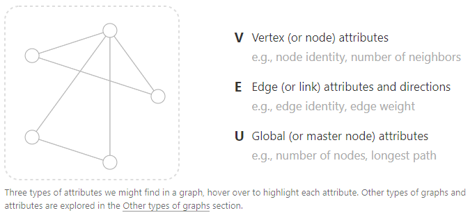
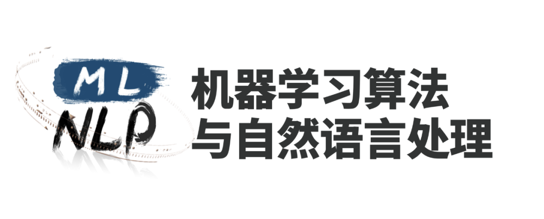
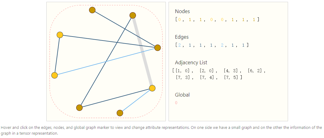
A graph consists of three parts: Vertex (V), Edge (E), and Global (U). V can be represented as node identity or the number of neighbors, E can be represented as edge identity or edge weight, and U can be represented as the number of nodes or the longest path. To further describe each node, edge, and entire graph, information can be stored in each part of the graph. Essentially, it is about storing information in an embedding manner.
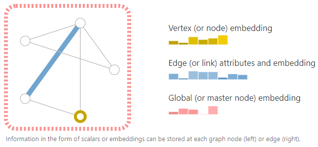
Special graphs can also be constructed through the directionality of edges (directed or undirected).
02Graphs and Where to Find Them Graph data is ubiquitous in life; for example, the most common images and text can be considered a special case of graph data, and there are other scenarios where graph data can be expressed.1. Images as Graphs
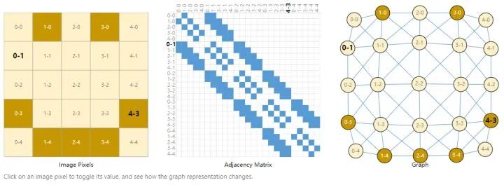
The position of an image can be represented in the form of (columns-rows), constructing the image into an adjacency matrix, where the blue blocks represent the adjacency between pixels, with no directionality. The graph representation is shown in the image on the right.2. Text as Graphs
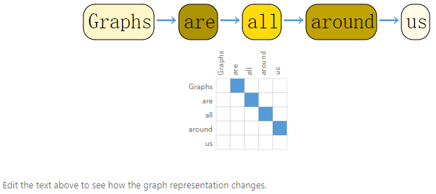
Text can also be constructed into an adjacency matrix; unlike images, text is a directed graph where each word is only connected to the previous word, and there is directionality. Other examples include molecules, social networks, academic citation networks, etc., which can also be constructed as graphs.02What Types of Problems Have Graph Structured Data? Graphs can handle three levels of problems: graph-level, node-level, and edge-level.1. Graph-level Task
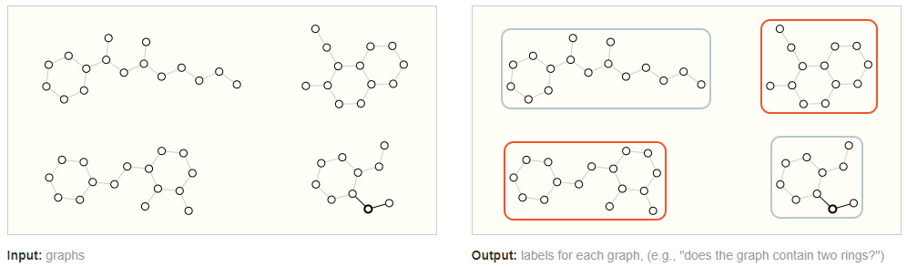
Input a graph and output the category of the entire graph. In images, this is similar to image classification tasks; in text, it is similar to sentence sentiment analysis.2. Node-level Task
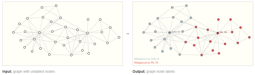
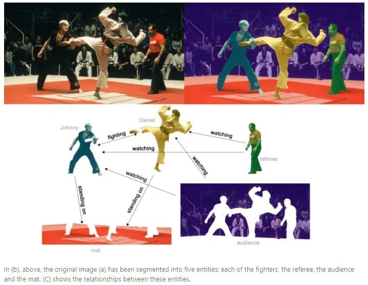
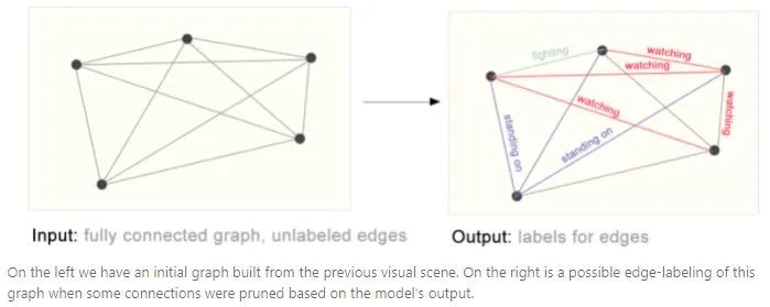
Input a graph with nodes that do not carry categories and output the category of each node. In images, this is similar to semantic segmentation; in text, it is similar to part-of-speech classification.3. Edge-level Task Edge-level tasks are used to predict the relationships between nodes. As shown in the figure below, first, different parts are segmented, and then the relationships between different parts are determined. Constructing a graph means predicting the category of edges.
4. The Challenges of Using Graphs in Machine Learning How to use neural networks to handle graph tasks? The first step is to consider how to represent graphs in a way that is compatible with neural networks. A graph can have up to four types of information to predict: node, edge, global-context, and connectivity. The first three are relatively easy, for example, one can represent the feature matrix N that stores the characteristics of the i-th node. However, representing connectivity is much more complex. The most straightforward way is to construct an adjacency matrix, but it is space-inefficient and may produce very sparse adjacency matrices. Another issue is that many adjacency matrices can encode the same connectivity but do not guarantee that these different matrices will produce the same results in neural networks (meaning they are not permutation invariant). A graceful and efficient way to represent sparse matrices is to use adjacency lists. Edge represents the connectivity between nodes, represented in the k-th item of the adjacency list as a tuple (i,j). For example, the adjacency list of a graph is shown in the figure below:
03Graph Neural Networks Through the description above, a graph can be represented using a permutation-invariant adjacency list, thus we can design a Graph Neural Network (GNN) to solve graph prediction tasks.1. The Simplest GNN
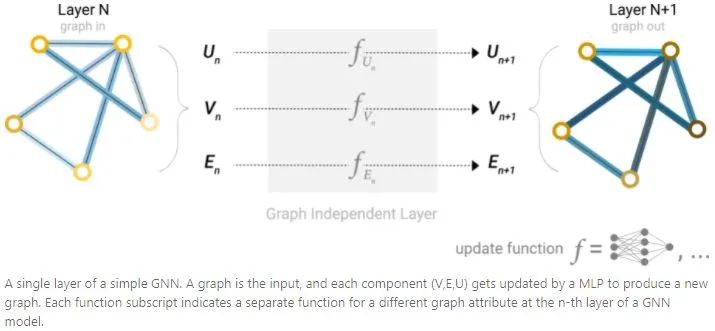
Starting with the simplest GNN, update the properties of all graphs (nodes (V), edges (E), global (U)) as new embeddings, but do not use the connectivity of the graph. GNN uses MLP separately for each component of the graph, termed GNN layer. For each node vector, after using MLP, it returns a learned node vector; similarly, edges will return a learned edge embedding, and global will return a global embedding. Similar to CNN, GNN layers can be stacked to form a GNN. Since GNN layers do not update the connectivity of the input graph, the output graph’s adjacency list remains the same as the input graph. However, through GNN layers, the embeddings of nodes, edges, and global-context have been updated.2. GNN Predictions by Pooling Information
If you want to use GNN for binary classification tasks, you can use a linear classifier to classify the graph.
However, sometimes information is only stored in edges, so it is necessary to collect information from edges to transfer to nodes for prediction. This process is called pooling. The pooling process has two steps: 1. For each item to be pooled (each column in the row of the above image), collect their embeddings and concatenate them into a matrix (the row in the above image). 2. The collected embeddings are aggregated through a summation operation.
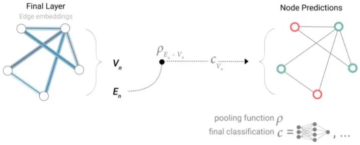
Therefore, if only edge-level features are available, information can be passed through pooling to predict nodes (the dotted line in the above image indicates that pooling passes information to nodes, which then perform binary classification).
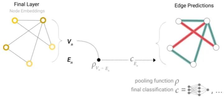
Similarly, if only node-level features are available, information can be passed through pooling to predict edges, similar to global average pooling in CV.
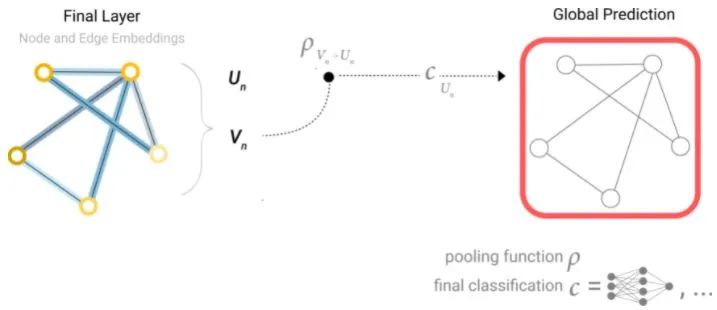
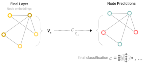
Similarly, global predictions can be made using node-level features.
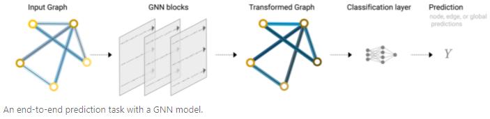
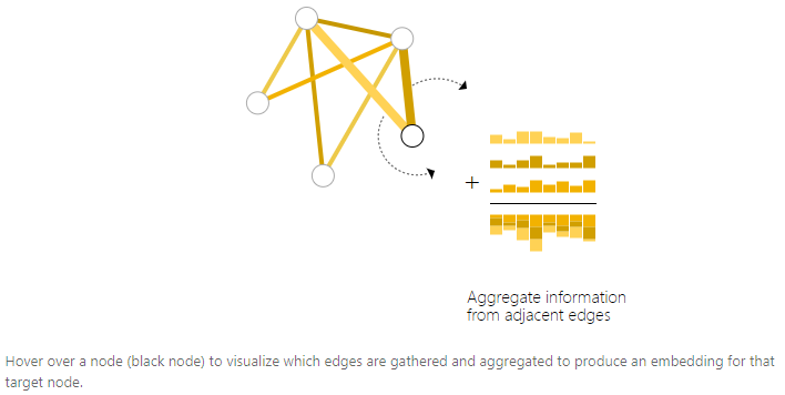
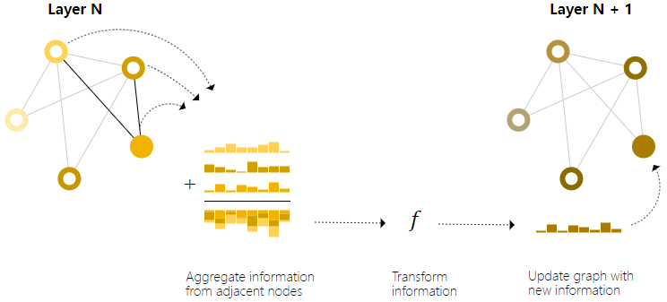
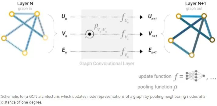
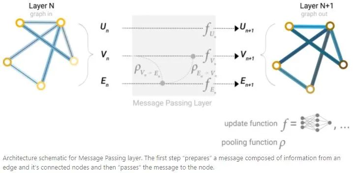
Similar to CNN, an end-to-end GNN can be constructed through GNN blocks. It is important to note that in this simplest GNN, the connectivity of the graph is not used in the GNN layer. Each node, edge, and global-context is processed independently, only using connectivity during the aggregation of information for prediction.3. Passing Messages Between Parts of the Graph To make learned embeddings aware of the connectivity of the graph, pooling can be used in the GNN layer to construct a more complex GNN (similar to convolution). Message passing can be implemented, allowing adjacent nodes or edges to exchange information and influence each other’s embedding updates. The message passing process consists of three steps: 1. For each node in the graph, collect the embeddings of all adjacent nodes. 2. Aggregate all messages through addition. 3. All aggregated messages are passed through an update function (usually a learnable neural network). These steps are key to utilizing the connectivity of the graph. By constructing more refined message passing variants in the GNN layer, more expressive and capable GNN models can be obtained.
Through stacked message passing GNN layers, a node can introduce information from the entire graph: after three layers of GNN, a node can obtain information from nodes three steps away. Updating the simplest GNN paradigm by adding a message passing operation:
4. Learning Edge Representations
Through message passing, information can be shared between nodes and edges in the GNN layer. Just like using information from adjacent nodes, edge information can be pooled first and then transformed and stored using an update function, aggregating information from adjacent edges. However, the information stored in nodes and edges in the graph may not have the same size or shape, so it is not immediately clear how to combine them. One method is to learn a linear mapping from the node space to the edge space, or one can concatenate them before the update function.
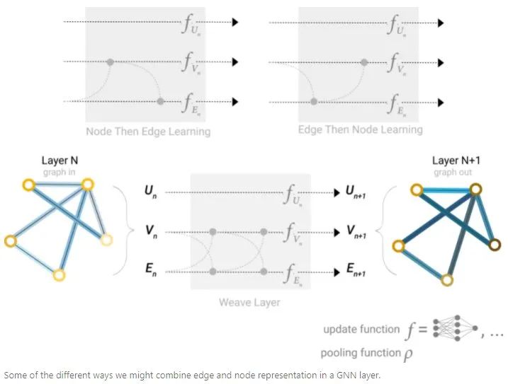
When constructing a GNN, it is necessary to design which graph properties to update and the order of updates. For example, one can use a weaving method for updates, node to node (linear), edge to edge (linear), node to edge (edge layer), edge to node (node layer).5. Adding Global Representations
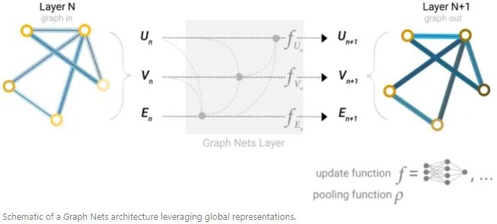
The GNN model described above has a flaw: nodes that are far apart in the graph cannot effectively transmit information. For a node, if there are k layers, the maximum distance for information transmission is k steps, which poses a serious problem for prediction tasks that rely on information from distant nodes. One solution is to allow all nodes to transmit information to each other, but for large graphs, this computation can be very expensive. Another solution is to use a global representation of the graph (U), called a master node or context vector. This global context vector can connect to all nodes and edges in the network and serve as a bridge for information transmission between them, constructing an overall representation of the graph.
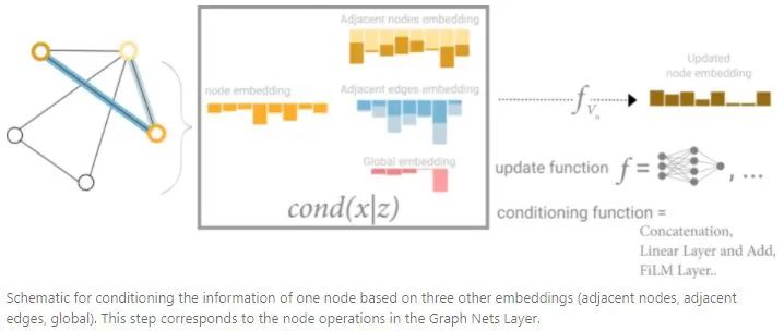
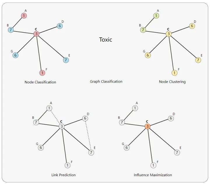
From this perspective, all graph properties can be utilized by associating the properties of interest with other properties and then leveraging them during the pooling process. For example, for a node, one can consider adjacent nodes, edges, and global information simultaneously, and then associate them through concatenation, finally mapping them into the same feature space through linear mapping.04The Challenges of Computation on Graphs There are three challenges in computing with graphs: lack of consistent structure, node-order equivariance, and scalability.1. Lack of Consistent Structure Graphs are extremely flexible mathematical models, which also means they lack consistent structure across instances. For example, different molecules have different structures. Representing graphs in a computable format is not trivial, and the final representation of a graph is often determined by the actual problem.2. Node-Order Equivariance Nodes in a graph typically do not have an intrinsic order, whereas in images, each pixel is uniquely determined by its absolute position in the image. Therefore, we want our algorithms to be node-order invariant: they should not depend on the order of nodes in the graph. If we somehow arrange the nodes, the node representations computed by the algorithm should also be arranged in the same way.3. Scalability Graphs can be very large, like social networks such as Facebook and Twitter, which have over a billion users, making operations on such large data challenging. Fortunately, most naturally occurring graphs are “sparse”: their number of edges often has a linear relationship with the number of vertices. The sparsity of graphs allows for special methods to efficiently compute node representations in graphs. Additionally, compared to the volume of graph data, these methods have far fewer parameters.04Problem Setting and Notation Many problems can be represented using graphs:Node Classification: Classifying individual nodes. Graph Classification: Classifying entire graphs. Node Clustering: Grouping similar nodes based on connectivity. Link Prediction: Predicting missing links. Influence Maximization: Identifying influential nodes.
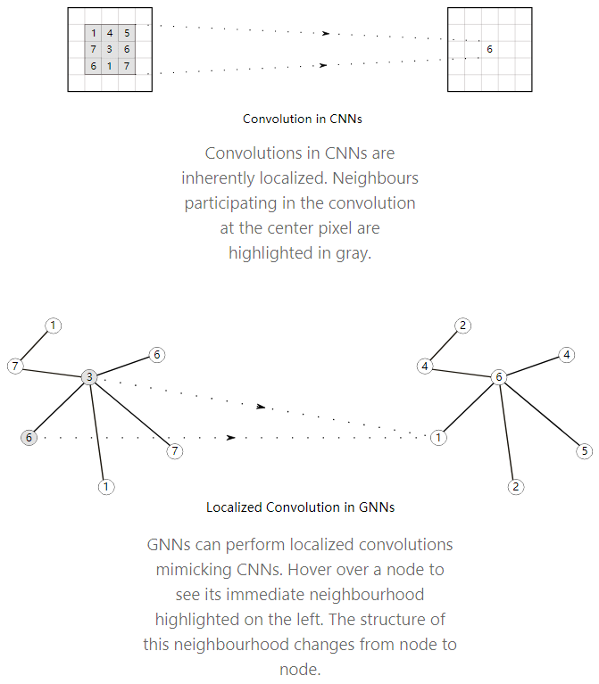
05Extending Convolutions to Graphs Convolutional neural networks are very powerful in extracting features from images. Images themselves can be seen as a very regular grid-like structure graph, where individual pixels are nodes, and the RGB channel values at each pixel are node features. Therefore, it is a natural idea to extend convolution to arbitrary graphs. However, ordinary convolutions are not node-order invariant because they depend on the absolute positions of pixels. Graphs can ensure consistent neighborhood structure for each node by performing some padding and sorting, but there are more universal and powerful methods to address this issue.
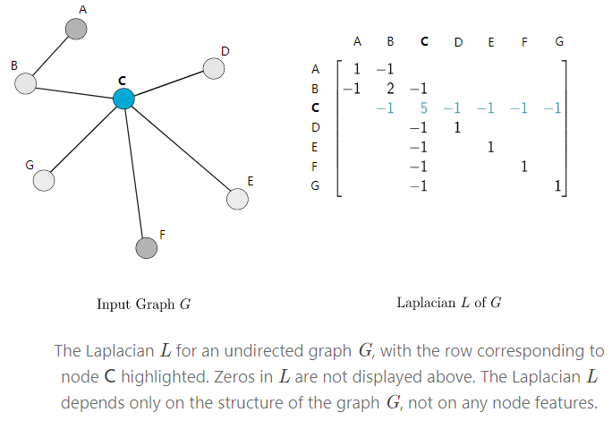
Below, we will first introduce how to construct polynomial filters on the node neighborhood, which is similar to filtering on adjacent pixels in CNNs. Then we will introduce more recent methods that use stronger mechanisms to extend this idea.06Polynomial Filters on Graphs1. The Graph Laplacian Given a graph G, let A represent the adjacency matrix with values of 0 or 1, and D represent the diagonal matrix (the diagonal values represent the number of neighboring nodes of the row node), then . The graph Laplacian matrix L can be expressed as: L=D – A. The right figure’s diagonal represents the degree of the row node, while the negative values are the subtracted adjacency matrix (the blue numbers correspond to C in the graph).
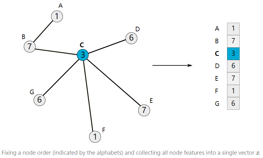
2. Polynomials of the Laplacian The polynomials of the Laplacian can be expressed as: These polynomials can be considered equivalent to “filters” in CNNs, where the coefficients w are the weights of the “filters”. For convenience, we will consider the case where nodes have only one-dimensional characteristics (each node is a value). Using the previously chosen node order, we can stack all node features to obtain a vector x.
By constructing the feature vector x, we can define the convolution formula of it with the polynomial filter as: Regarding how the Laplacian matrix acts on x, refer to https://distill.pub/2021/understanding-gnns/.3. ChebNet ChebNet improves the polynomial filter formula: where is the first Chebyshev polynomial of degree i, and is the normalized Laplacian matrix defined using the maximum eigenvalue of L. For details on ChebNet, refer to https://distill.pub/2021/understanding-gnns/.4. Embedding Computation Below, we will introduce how to stack nonlinear ChebNet (or any polynomial filter) layers to construct a GNN, just like a standard CNN. Suppose there are K different polynomial filter layers, the learnable parameters of are represented as , then the computation process can be expressed as:
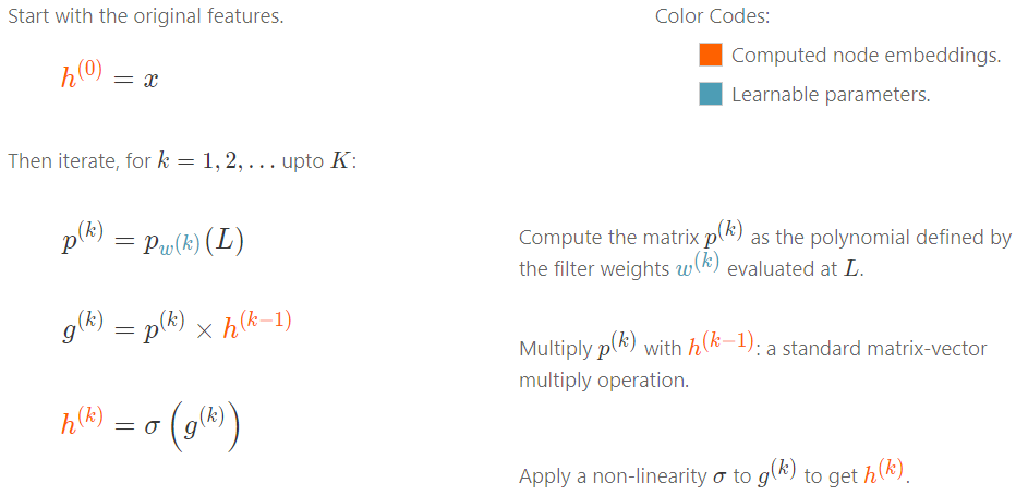
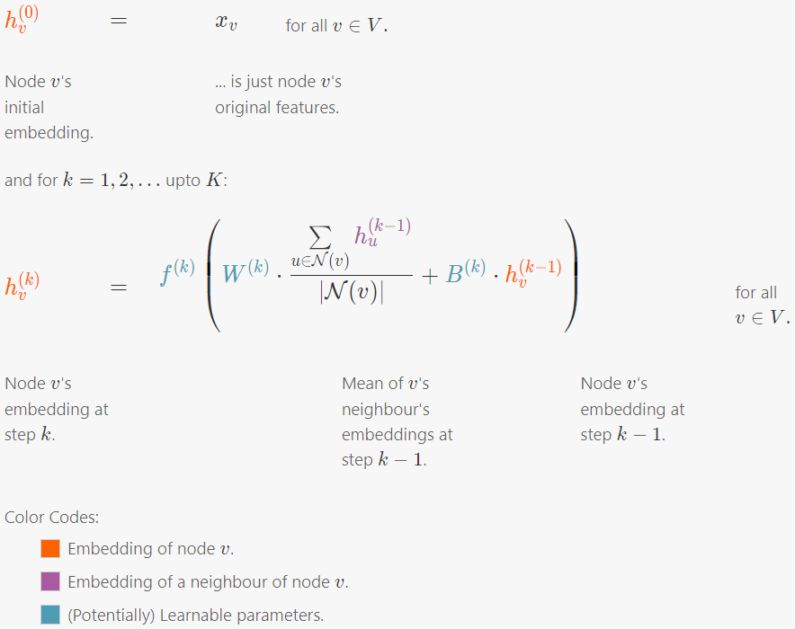
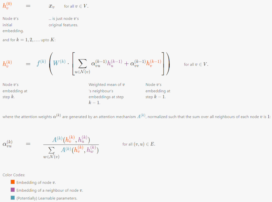
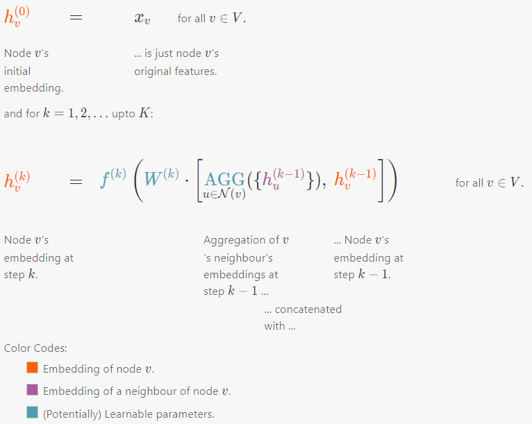
GNNs and CNNs have similar computation methods, taking input as initial features, then computing polynomial filters, and finally performing matrix multiplication with input features, followed by a nonlinear transformation with a nonlinear function, iterating K times. It is important to note that GNNs share filter weight parameters across different nodes, similar to CNNs, where convolution parameters are also shared across different positions.07Modern Graph Neural Networks ChebNet is a breakthrough in learning local filters in graphs, inspiring many to think about graph convolution from different angles. Polynomial filters can be expanded as: this is actually a 1-step local convolution (that is, convolution only with directly connected nodes), which can be seen as generated by two steps: 1. Aggregating features from directly adjacent nodes. 2. Combining the features of the node itself. By ensuring that aggregation is node-order equivariant, the entire convolution can be guaranteed to be node-order equivariant. These convolutions can be seen as “message passing” between adjacent nodes: after each step, each node receives information from its neighboring nodes. By iteratively repeating the 1-step local convolution K times, the receptive field encompasses all nodes up to K steps away.1. Embedding Computation Message passing forms the backbone of many GNN models. Below are some popular GNN models:
-
Graph Convolutional Networks (GCN)
-
Graph Attention Networks (GAT)
-
Graph Sample and Aggregate (GraphSAGE)
-
Graph Isomorphism Network (GIN)
2. GCN
3. GAT
4. GraphSAGE
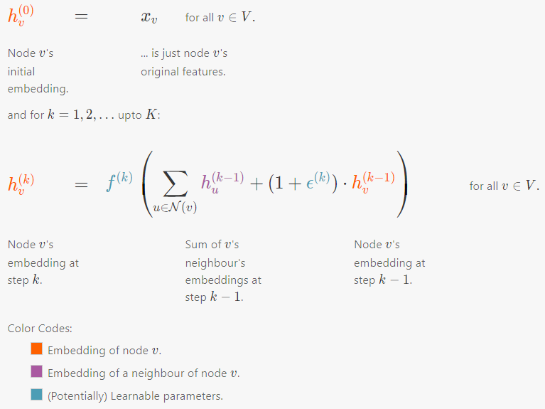
5. GIN
Comparing GCN, GAT, GraphSAGE, and GIN, the main differences lie in how information is aggregated and how it is transmitted.08Conclusion This article provides a brief introduction to some variants of GNN and GCN, but the field of graph neural networks is extremely vast. Here are some points that may be of interest: GNNs in Practice: How to improve the efficiency of GNNs, regularization techniques for GNNs Different Kinds of Graphs: Directed graphs, Temporal graphs, Heterogeneous graphs Pooling: SortPool, DiffPool, SAGPool
About Us
MLNLP(Machine Learning Algorithms and Natural Language Processing) is a grassroots academic community jointly built by scholars in natural language processing from home and abroad. It has developed into one of the largest natural language processing communities in China and abroad, gathering over 500,000 subscribers, and includes well-known brands such as Top Conference Exchange Group, AI Selection, AI Talent Exchange, and AI Academic Exchange, aimed at promoting progress between the academic and industrial sectors of machine learning and natural language processing and enthusiasts.The community can provide an open communication platform for relevant practitioners’ further education, employment, and research. Everyone is welcome to follow and join us.