Source: AI Snail Car, Extreme City Platform


This article is about 9200 words long, and it is recommended to read for more than 10 minutes.
This article briefly introduces several common CNN optimization methods and shares relevant experiences.

Author | Li Ming Huai JinSource | https://zhuanlan.zhihu.com/p/80361782

Introduction

Convolution is one of the core computations in neural networks, and its groundbreaking progress in computer vision has led to the boom of deep learning. There are many variants of convolution, and its computational complexity is high. Most of the time in neural network execution is spent on convolution computation, and the continuous development of network models is increasing the depth of networks, making it particularly important to optimize convolution computations.With the development of technology, researchers have proposed various optimization algorithms, including Im2col, Winograd, etc. This article first defines the concept of convolutional neural networks, then briefly introduces several common optimization methods, and discusses some experiences of the author in this field.

• Most of the time is spent on computing convolutions link:https://arxiv.org/abs/1807.11164
• Im2col link:https://www.mathworks.com/help/images/ref/im2col.html
• Winograd link:https://www.intel.ai/winograd/#gs.avmb0n

Concept of Convolutional Neural Networks

The concept of Convolutional Neural Networks (CNN) is an extension of convolution from the field of signal processing. The convolution in signal processing is defined as (1)Due to symmetry 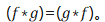Convolution calculations are intuitively not easy to understand, as visualized in Figure 1. The red slider in the figure moves and the triangle pattern drawn by the product with the blue square is the convolution result (𝑓∗𝑔)(𝑡) at various points.

Figure 1: Convolution in Signal Processing

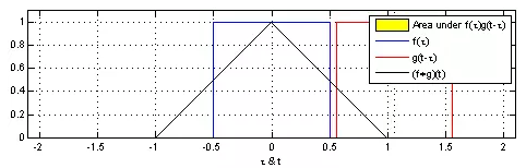
• Link to convolution in signal processing:https://jackwish.net/convolution-neural-networks-optimization.html

The discrete form of Formula 1 is: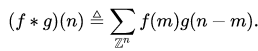(2)Expanding this convolution to two-dimensional space gives the convolution in neural networks, which can be abbreviated as: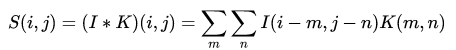(3)Where 𝑆 is the convolution output, 𝐼 is the convolution input, and 𝐾 is the convolution kernel. The dynamic visualization of this calculation can refer to conv_arithmetic, which will not be introduced here.

• Link to conv_arithmetic:https://github.com/vdumoulin/conv_arithmetic

When applied to computer vision for image processing, the channels of the image can simply stack two-dimensional convolutions as follows: (4)Where 𝑐c is the input channel. This is how two-dimensional convolution is applied in three-dimensional tensors.Many times, formula descriptions seem not very intuitive, and Figure 2 visualizes the stacked two-dimensional convolution. Among them, the labels related to inputs, outputs, and convolution kernels are prefixed with I, O, K. In addition, the colors used in this article for output, input, and convolution kernels are generally: orange, yellow, and green.

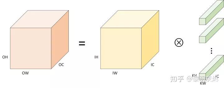
Figure 2: Definition of Convolution CalculationIn this case, the memory layout of the tensor is NHWC, and the corresponding pseudocode for convolution calculation is as follows. The outer three loops traverse each data point of the output 𝐶C, and for each output data, the inner three loops need to accumulate sums to obtain (the dot product).

for (int oh = 0; oh < OH; oh++) {for (int ow = 0; ow < OW; ow++) {    for (int oc = 0; oc < OC; oc++) {      C[oh][ow][oc] = 0;      for (int kh = 0; kh < KH, kh++){        for (int kw = 0; kw < KW, kw++){          for (int ic = 0; ic < IC, ic++){            C[oh][ow][oc] += A[oh+kh][ow+kw][ic] * B[kh][kw][ic];          }        }      }    }  }}

Optimization Methods Similar to Matrix MultiplicationWe can also perform basic optimization operations such as vectorization, parallelization, and loop unrolling for this computation. The problem with convolution is that its 𝐾𝐻 and 𝐾𝑊 are generally not more than 5, making it difficult to vectorize, while the computation of features has data reuse in the spatial dimension. The complexity of this calculation has led to several optimization methods, which we will introduce below.

• Link to optimization methods similar to matrix multiplication:https://jackwish.net/gemm-optimization.html

Im2col Optimization Algorithm

As an early deep learning framework, the implementation of convolution in Caffe uses the im2col-based method, which is still one of the important optimization methods for convolution today.Im2col is the process of converting images into matrix columns in the field of computer vision. From the introduction in the previous section, it can be seen that the calculation of two-dimensional convolution is relatively complex and not easy to optimize. Therefore, in the early development of deep learning frameworks, Caffe used the Im2col method to convert three-dimensional tensors into two-dimensional matrices, thereby fully utilizing the already optimized GEMM libraries to accelerate convolution calculations for various platforms. Finally, the two-dimensional matrix results obtained from matrix multiplication are converted back to three-dimensional matrices using Col2im.

• Caffe link:http://caffe.berkeleyvision.org/
• Caffe uses Im2col method to convert three-dimensional tensors into two-dimensional matrices link:https://github.com/Yangqing/caffe/wiki/Convolution-in-Caffe:-a-memo

Algorithm Process

Unless otherwise specified, the memory layout form used in this article is assumed to be NHWC. Other memory layouts and specific transformed matrix shapes may differ slightly but do not affect the description of the algorithm itself.

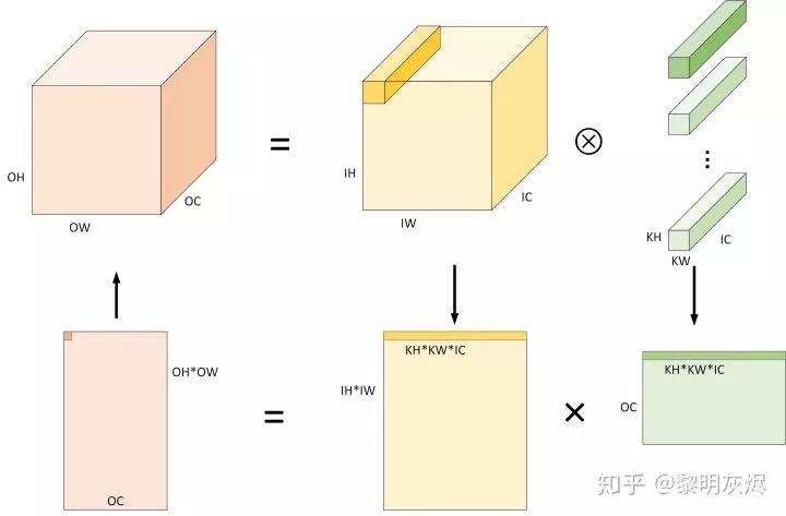
Figure 3: The Process of Calculating Convolution Using Im2col AlgorithmFigure 3 is an example of the process of calculating convolution using the Im2col algorithm. The specific process includes (for simplicity, ignoring the case of Padding, that is, assuming 𝑂𝐻=𝐼𝐻,𝑂𝑊=𝐼𝑊):

1. Expanding the input from 𝐼𝐻×𝐼𝑊×𝐼𝐶 into a two-dimensional matrix of shape (𝑂𝐻×𝑂𝑊)×(𝐾𝐻×𝐾𝑊×𝐼𝐶) based on the characteristics of convolution computation. Obviously, the memory space used after conversion is about 𝐾𝐻∗𝐾𝑊−1 times more than the original input.
2. The shape of the weights is generally a four-dimensional tensor of 𝑂𝐶×𝐾𝐻×𝐾𝑊×𝐼𝐶, which can be directly processed as a two-dimensional matrix of shape (𝑂𝐶)×(𝐾𝐻×𝐾𝑊×𝐼𝐶)).
3. For the two prepared two-dimensional matrices, running matrix multiplication can obtain an output matrix of shape (𝑂𝐻×𝑂𝑊)×(𝑂𝐶) by using (𝐾𝐻×𝐾𝑊×𝐼𝐶) as the dimension for accumulation and summation.
4. The output matrix (𝑂𝐻×𝑂𝑊)×(𝑂𝐶) in terms of memory layout is the expected output tensor 𝑂𝐻×𝑂𝑊×𝑂𝐶.

The cost of using GEMM for convolution with Im2col is the extra memory overhead. This is because in the original convolution calculation, the convolution kernel slides over the input to compute the output, and adjacent output calculations reuse certain inputs in space. When using Im2col to flatten the three-dimensional tensor into a two-dimensional matrix, these originally reusable data are flattened and spread across the matrix, leading to 𝐾𝐻∗𝐾𝑊−1 copies of the input data.When the size of the convolution kernel 𝐾𝐻×𝐾𝑊 is 1×1, the 𝐾𝐻 and 𝐾𝑊 in the above steps can be eliminated, meaning that the shape of the converted input is (𝑂𝐻×𝑂𝑊)×(𝐼𝐶), the shape of the convolution kernel is (𝑂𝐶)×(𝐼𝐶), and the convolution calculation degenerates into matrix multiplication. It is worth noting that for this case, the Im2col process does not actually change the shape of the input, so the matrix multiplication operation can be directly performed on the original input, thus saving the process of memory organization (i.e., steps 1, 2, and 4 in the above).

Memory Layout and Convolution Performance

The memory layout of convolutions in neural networks mainly includes NCHW and NHWC. Different memory layouts will affect the access patterns to memory during computation, especially when running matrix multiplication. This section analyzes the relationship between computational performance and memory layout when using the Im2col optimization algorithm.

• Link to the performance of matrix multiplication:https://jackwish.net/gemm-optimization.html

After completing the Im2col transformation, input matrices and convolution kernel matrices for running matrix multiplication are obtained. Common data partitioning, vectorization, and other optimization methods used in matrix calculations are applied to the computation process (for relevant definitions, please refer to General Matrix Multiplication (GEMM) Optimization Algorithm). Below, we focus on analyzing the impact of different memory layouts on performance in this context.

• Link to General Matrix Multiplication (GEMM) Optimization Algorithm:https://jackwish.net/gemm-optimization.html

First, consider the NCHW memory layout. The convolution corresponding to the NCHW memory layout is related to matrix multiplication 𝐶=𝐴𝐵, where 𝐴 is the convolution kernel (filter), and 𝐵 is the input (input). The dimensions of each matrix are shown in Figure 4. In the figure, 𝑀,𝑁,𝐾 are used to denote the matrix multiplication, that is, 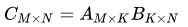, and their relationships with various dimensions in convolution calculations are marked in the figure.

Figure 4: Matrix Multiplication Converted from NCHW Memory Layout ConvolutionAfter partitioning this matrix, we analyze the performance of locality in detail, which is marked in Figure 4. Inside indicates the locality within the 4×4 small block matrix multiplication, while Outside indicates the locality between small blocks in the dimension reduction direction.

• For output, the locality within the small block is poor because each vectorized load will load four elements, and each load will cause a cache miss. The external performance depends on the global computation direction—row-major order has better locality, while column-major order has poorer locality. The behavior of output is not the endpoint of the discussion here, as it has no memory reuse.
• For the convolution kernel, the locality within the small block is poor, similar to output. When small block loading causes cache misses, the processor will load a cache line at once, allowing several subsequent small block accesses to hit the cache (Cache hit) until the entire cache line is hit before entering the next cache line range. Therefore, the external locality of small blocks is good.
• For input, the locality within the small block is also poor. However, unlike the convolution kernel, the cache line data loaded into the cache within the small block due to cache misses will only be used once because the address range of the next small block generally exceeds one cache line. Therefore, almost every memory load of input will result in a cache miss—the cache does not play a role in accelerating, and each memory access needs to fetch data from memory.

Thus, when processing convolution calculations with Im2col, the NCHW layout is not memory-friendly.Figure 5 is an example of the NHWC memory layout. It is worth noting that in NHWC and NCHW, the matrices 𝐴 and 𝐵 represent different tensors—𝑂𝑢𝑡𝑝𝑢𝑡=𝐼𝑛𝑝𝑢𝑡×𝐹𝑖𝑙𝑡𝑒𝑟 (the swap is just to avoid drawing another figure). The specific partitioning method is still the same, and it is the matrix constructed in the steps described in the previous section.

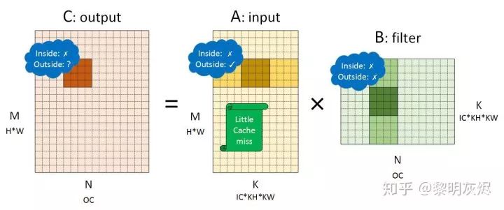
Figure 5: Matrix Multiplication Converted from NHWC Memory Layout ConvolutionSimilarly, analyzing the memory performance of the three tensors shows:

• For output, NHWC and NCHW perform the same.
• For input, the locality within small blocks is not good because several vector loads will cause cache misses; however, the external locality performs well because the memory used in the dimension reduction sliding is contiguous. This performance is similar to that of the convolution kernel in NCHW, overall, it is a memory layout that is friendly to the cache.
• For the convolution kernel, the situation in NHWC is similar to that of input in NCHW; both internal and external locality are poor.

In both memory layouts, the cache performance of the convolution kernel is not an issue because the convolution kernel remains unchanged during execution, and the memory layout of the convolution kernel can be rearranged during the model loading phase to make it cache-friendly in the memory outside the small block (for example, converting the layout of (𝐼𝐶×𝐾𝐻×𝐾𝑊)×(𝑂𝐶) to (𝑂𝐶)×(𝐼𝐶×𝐾𝐻×𝐾𝑊)). It is worth noting that the execution of general frameworks or engines can generally be divided into two phases: preparation phase and execution phase. Some preprocessing work of the model can be completed in the preparation phase, such as rearranging the memory layout of the convolution kernel, which is data that remains unchanged during the execution phase.Therefore, when using the Im2col method for calculations, the overall memory performance depends on the input situation, meaning that the NHWC memory layout is more friendly than the NCHW memory layout. An experiment we conducted during the practical process showed that for a 1×1 convolution kernel, when similar optimization methods are used, converting from NCHW to NHWC can reduce the cache miss rate from about 50% to around 2%. This level of improvement can significantly enhance software performance (here referring specifically to cases where specially designed matrix multiplication optimization methods are not used).

Spatial Packing Optimization Algorithm

Im2col is a relatively naive convolution optimization algorithm that can lead to large memory overhead if not carefully handled. Spatial packing is an optimization algorithm similar to matrix multiplication memory reorganization.

• Link to matrix multiplication memory reorganization:https://github.com/flame/how-to-optimize-gemm/wiki#packing-into-contiguous-memory

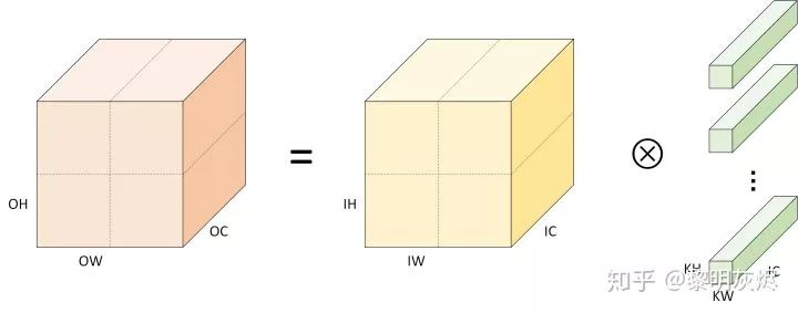
Figure 6: Division of Computation by Spatial Packing Optimization AlgorithmSpatial packing optimization algorithm is a method based on the divide and conquer approach—it divides convolution calculations into several parts based on spatial characteristics and processes them separately. Figure 6 shows the spatial division of outputs and inputs into four parts.After partitioning, a large convolution calculation is broken down into several smaller convolution calculations. Although the total amount of computation remains unchanged during the partitioning process, the locality of memory access during small matrix calculations is better, allowing performance improvements through the computer’s storage hierarchy. This is accomplished through the steps shown in Figure 7. The process is similar to the memory reorganization process of Im2col described in the previous section:

1. In the H and W dimensions, the input tensor of shape 𝑁×𝐻×𝑊×𝐼 is divided into ℎ∗𝑤 parts (splitting ℎ and 𝑤 times in two directions), and these small tensors are organized into contiguous memory;
2. Perform two-dimensional convolution operations between the ℎ∗𝑤 obtained input tensors and the convolution kernel to obtain ℎ∗𝑤 output tensors of shape 𝑁×𝐻/ℎ×𝑊/𝑤×𝑂𝐶;
3. Reorganize the memory layout of these output tensors to obtain the final shape of 𝑁×𝐻×𝑊×𝑂𝐶.

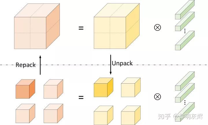
Figure 7: Steps of Spatial Packing CalculationIt is worth noting that for convenience, the Padding issue has been ignored in the above description. In practice, when partitioning the input tensor into several small tensors in step 1, in addition to copying the original data in the partitioned small blocks, it is also necessary to copy the boundary data of adjacent small tensors. Specifically, as shown in Figure 8, the shape of the small tensors obtained from spatial splitting is actually:𝑁×(𝐻/ℎ+2(𝐾𝐻−1))×(𝑊/𝑤+(𝐾𝑊−1))×𝐶.(5)Here, the 2(𝐾𝐻−1) and 2(𝐾𝑊−1) follow the Padding rules. The rules arewhen they can be ignored; and the rule is SAME when the Padding at the boundary of the source tensor must be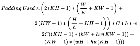, while the Padding not at the boundary of the source tensor uses the values of neighboring tensors. This is evident when considering the principles of convolution calculations.

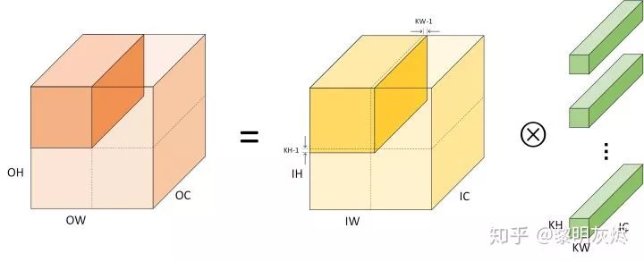
Figure 8: Details of Spatial Packing Algorithm DivisionThe above three example figures are all cases divided into 4 parts. In practical applications, they can be divided into many parts. For example, they can be divided into small tensors with a side length of 4 or 8, making it easier for the compiler to vectorize computational operations. As the partitioned tensors become smaller, their locality increases, but the downside is that the additional memory consumed also increases. This additional memory is due to the introduction of Padding. When divided into ℎ∗𝑤h∗w parts, the additional memory consumed by Padding is:As can be seen, as the granularity of the split becomes finer, the extra memory consumed increases. It is worth noting that when splitting to the finest granularity, i.e., dividing the output of shape 𝑁×𝐻×𝑊×𝑂𝐶 into 𝐻∗𝑊 parts, the spatial packing degenerates into the Im2col method. At this point, the convolution at one element is equivalent to the dot product of matrix multiplication when calculating an output element.When only performing spatial partitioning, the partitioning is independent of the convolution kernel. However, if partitioning is done in the output channel dimension, the convolution kernel can also be split accordingly. The partitioning in the channel dimension is equivalent to simple stacking after fixing the spatial partitioning, which does not affect memory consumption but will impact locality. Finding a suitable partitioning method for different scales of convolution is not an easy task. Like many problems in the field of computer science, this problem can also be automated; for example, AutoTVM can find optimal partitioning methods under such circumstances.AutoTVM link:https://arxiv.org/abs/1805.08166

Winograd Optimization Algorithm

The two algorithms introduced in the previous sections, Im2col calls the GEMM computation library after organizing three-dimensional tensors into matrices, and spatial packing optimization itself utilizes locality optimization methods. The Winograd optimization algorithm introduced in this section is an application of the Coppersmith–Winograd algorithm among matrix multiplication optimization methods and is based on algorithm analysis methods.This section contains many formulas, which are inconvenient for typesetting. If you are interested, please refer to the original text or other related literature.

Link to the original text:

https://jackwish.net/convolution-neural-networks-optimization.html

Indirect Convolution Optimization Algorithm

Marat Dukhan introduced the Indirect Convolution Algorithm in QNNPACK (Quantized Neural Network PACKage), which seems to be the fastest among all publicly available methods as of mid-2019. Recently, the author published related articles to introduce the main ideas.Although the implementation of this algorithm in QNNPACK is mainly used for quantized neural networks (other quantization optimization schemes in the industry are relatively traditional, such as TensorFlow Lite using Im2col optimization algorithm, Tencent’s NCNN using Winograd optimization algorithm; OpenAI’s Tengine using Im2col optimization algorithm), it is also a similar optimization algorithm design.At the time of writing this article, the design of the article had not been made public, and it is best to understand many details of the algorithm design in conjunction with the code. My QNNPACK fork contains an explained branch, which includes comments on some of the code for reference.

QNNPACK link:

https://github.com/pytorch/QNNPACK

TensorFlow Lite using Im2col optimization algorithm link:

https://github.com/tensorflow/tensorflow/blob/v2.0.0-beta1/tensorflow/lite/kernels/internal/optimized/integer_ops/conv.h

NCNN using Winograd optimization algorithm link:

https://github.com/Tencent/ncnn/blob/20190611/src/layer/arm/convolution_3x3_int8.h

Tengine using Im2col optimization algorithm link:

https://github.com/OAID/Tengine/blob/v1.3.2/executor/operator/arm64/conv/conv_2d_fast.cpp

My QNNPACK fork link:

https://github.com/jackwish/qnnpack

Computational Workflow

The effective operation of the indirect convolution algorithm relies on a key premise—during continuous network operation, the memory address of the input tensor remains unchanged. This characteristic is relatively easy to satisfy; even if the address needs to change, it can be copied to a fixed memory area.

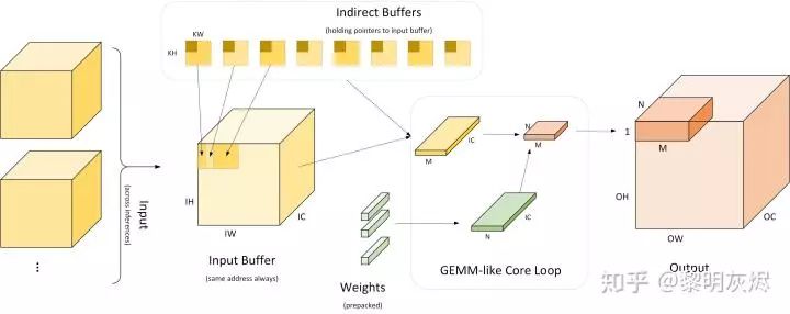
Figure 9: Workflow of Indirect Convolution AlgorithmFigure 9 details the workflow of the indirect convolution algorithm. The leftmost part indicates that multiple inputs use the same input buffer (Input Buffer). The indirect convolution algorithm builds an “indirect buffer” (Indirect Buffer) based on this input buffer, which is the core of the indirect convolution algorithm. As shown on the right side of the figure, during network operation, each time an output of size 𝑀×𝑁 is computed, where 𝑀 treats 𝑂𝐻×𝑂𝑊 as a one-dimensional vector scale. Generally, 𝑀×𝑁 is 4×4, 8×8, or 4×8. When calculating the output of size 𝑀×𝑁, corresponding inputs are taken from the indirect buffer, and weights are also retrieved to compute the result. The calculation process is equivalent to calculating 𝑀×𝐾 and 𝐾×𝑁 matrix multiplication.In implementation, the execution process of the software is divided into two parts:

1. Preparation phase: Load the model, configure the input buffer; rearrange weights to make their memory layout suitable for subsequent calculations;
2. Execution phase: For each input, run ⌈𝑂𝐻∗𝑂𝑊/𝑀⌉∗⌈𝑂𝐶/𝑁⌉ core loops, calculating the output of size 𝑀×𝑁 each time using the GEMM method.

Figure 10: Indirect BufferAs discussed in related sections, the Im2col optimization algorithm has two issues: first, it occupies a lot of extra memory, and second, it requires additional data copying for the input. How can these two points be resolved? The indirect convolution algorithm provides the answer through the indirect buffer (Indirect Buffer), as shown on the right side of Figure 10.Figure 10 compares the conventional Im2col optimization algorithm with the indirect convolution optimization algorithm. As introduced in related sections, the Im2col optimization algorithm first copies the input to a matrix, as indicated by the relevant arrows in the Input section of Figure 10, and then performs matrix multiplication. The indirect convolution optimization algorithm uses the indirect buffer to store pointers to the input (which is also the reason why the indirect convolution optimization algorithm requires the input memory address to be fixed). During operation, the corresponding inputs can be simulated based on these pointers, similar to the matrix calculation process of Im2col.

Indirect Buffer Layout

The indirect buffer can be understood as a set of buffers the size of the convolution kernel, with a total of 𝑂𝐻×𝑂𝑊 buffers, each buffer being 𝐾𝐻×𝐾𝑊 in size—each buffer corresponds to the address of the input used for a certain output. For each spatial position output, one indirect buffer is used; outputs with the same spatial position but different channels use the same indirect buffer, and each pointer in the buffer is used to index the 𝐼𝐶 elements in the input. During computation, as the output moves, different indirect buffers are selected to obtain the corresponding input addresses. There is no need to calculate the addresses of the input to be used based on the coordinates of the output target, which is equivalent to pre-computing the addresses.Figure 11 illustrates the actual usage method and calculation process of the indirect buffer when 𝑀×𝑁 is 4, and both 𝐾𝐻 and 𝐾𝑊 are 3. The term local indirect buffer indicates that the current consideration is the core calculation process for computing 𝑀×𝑁.When calculating the output of size 𝑀×𝑁, the input used is the area covered by the convolution kernel sliding over the corresponding input position, which is of scale (𝐾𝐻)×(𝑀+2(𝐾𝑊−1))×𝐼𝐶. In the indirect convolution algorithm, these input memories are indexed by pointers in the 𝑀 indirect buffers, totaling 𝑀×𝐾𝐻×𝐾𝑊 pointers. Figure 11 identifies the corresponding relationship between the input spatial position in the upper left corner and the corresponding input buffer. It can be seen that the four input buffers A, B, C, and D correspond to the input addresses of adjacent two buffers with a difference of (𝐾𝑊−𝑆𝑡𝑟𝑖𝑑𝑒)/𝐾𝑊, which is 2/3 here, and the coordinates of the pointers in each buffer are also marked.

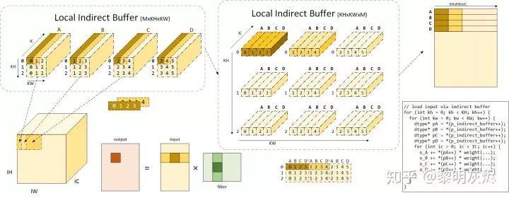
Figure 11: Explanation of Indirect BufferThe planar buffer in the figure is depicted in three-dimensional form (adding the IC dimension) to illustrate that each pointer in the indirect buffer can index 𝐼𝐶 input elements, and the contents indexed by each indirect buffer correspond to the input memory area associated with the weights.Furthermore, the arrangement of the upper left input buffer is not the final arrangement; in fact, these pointers will be processed into the form of the indirect buffer in the middle of Figure 11. By scattering the pointers in each buffer on the upper left, 𝐾𝐻×𝐾𝑊 pointers can be obtained; by collecting the pointers from different spatial positions of buffers A, B, C, and D, the arrangement of buffers in the upper part of the figure can be obtained, which is 𝐾𝐻×𝐾𝑊×𝑀. It can be seen that the pointers in the same spatial position of buffers A, B, C, and D are organized together. The upper part of the figure is the visual effect, while the lower part is the actual organization of the indirect buffer. The brown and dark yellow coloring in the figure corresponds to the same input memory or pointers. It is worth noting that the Stride in the legend is 1; when Stride is not 1, the coordinates of A, B, C, D in the same spatial position after reorganization may not be contiguous, and the adjacent spatial positions may differ by the size of the Stride.

Using Indirect Buffer for Computation

We have learned about the organization of the indirect buffer and the corresponding input memory addresses; now we will study how to use these buffers during the computation process.As in the previous section, the discussion in this section generally focuses on calculating outputs of size 𝑀×𝑁, which require 𝑀 inputs of size 𝐾𝐻×𝐾𝑊, among which there is data reuse. Now, reviewing the Im2col algorithm (as indicated in the lower left part of Figure 11), when vectorized to run calculations for the 𝑀×𝑁 matrix multiplication, each time 𝑀×𝑆 inputs of size and 𝑆×𝑁 weights are retrieved to run matrix multiplication on that block to obtain the corresponding partial sum result. Here, 𝑆 is the stepping factor for vectorized computation in the 𝐾 dimension.Essentially, the reason convolution can use the Im2col optimization algorithm is that its breakdown ignores the memory reuse, and the calculation process is equivalent to matrix multiplication. The indirect buffer allows simulating memory access to the input through pointers. When running the micro kernel for calculating outputs of size 𝑀×𝑁, 𝑀 pointers are used to scan the input. Each of the 𝑀 pointers retrieves 𝑀 addresses from the structure of the indirect buffer in the lower part of Figure 11, corresponding to the input memory of size 𝑀×𝐼𝐶, as shown in the upper right layout of the figure. In this stepping process, it still runs in the form of 𝑀×𝑆, where 𝑆 moves in the 𝐼𝐶 dimension. After this part of input scanning is completed, these 𝑀 pointers retrieve the corresponding pointers from the indirect buffer and continue the next traversal of the 𝑀×𝐼𝐶 input memory, calculating a partial sum of 1/(𝐾𝐻∗𝐾𝑊) each time. After this process runs 𝐾𝐻×𝐾𝑊 times, the output of size 𝑀×𝑁 is obtained. The pseudocode corresponding to this process is shown in the lower right corner of Figure 11. Since the indirect buffer has already been organized into a specific shape, every time the 𝑀 pointers are updated, they only need to be retrieved from the indirect buffer pointers (as indicated in the pseudocode in the figure under p_indirect_buffer).This process logic can be difficult to understand, so here is a bit of additional explanation. When the above 𝑀 pointers continuously move to scan memory, they are actually scanning the three-dimensional input after Im2col. The specificity of the input buffer is that it transforms the scanning of a two-dimensional matrix into the scanning of a three-dimensional tensor. The scanning process of the input corresponds to the scanning of the visualized input in the upper part of Figure 11. Connecting the corresponding input relationships between the upper left and lower left, it is easy to see that it scans the memory of size 𝑀×𝐼𝐶 in the input each time. It is worth noting that here, 𝑀×𝐼𝐶 consists of 𝑀 tensors of size 1×𝐼𝐶, and the spacing in the 𝑊 dimension is equal to the Stride.Thus, by running the core calculation ⌈𝑂𝐻∗𝑂𝑊/𝑀⌉∗⌈𝑂𝐶/𝑁⌉ times, all outputs can be obtained.The indirect convolution optimization algorithm solves three problems in convolution calculations: first, the spatial vectorization problem; second, the complexity of address calculations; third, the memory copying problem. Generally, convolution calculations require zero-padding for inputs (for cases where 𝐾𝐻×𝐾𝑊 is not 1×1). Traditional methods will incur memory copies during this process. However, the indirect buffer in the indirect convolution optimization algorithm cleverly solves this problem through indirect pointers. When constructing the indirect buffer, an additional 1×𝐼𝐶 memory buffer is created and filled with zero values. For spatial positions that require zero-padding, the corresponding indirect pointers are directed to this buffer, so that subsequent calculations are equivalent to already having zero-padding. For example, the upper left corner of A corresponds to the input spatial position (0,0); when zero-padding is required, this position must be zero value. At this point, only modifying the address of the indirect buffer is necessary.

Discussion, Summary, and Outlook

So far, this article has explored some published or open-source optimization methods for convolutional neural networks. These optimization methods have somewhat promoted the application of deep learning technology in the cloud or mobile end, helping our daily lives. For example, the garbage classification problem that recently troubled people in Shanghai and even all over China can also utilize deep learning methods to help people understand how to classify.

• Link to utilizing deep learning methods to help people understand classification:https://news.mydrivers.com/1/633/633858.htm

From the concentrated optimization methods in this article, it can be seen that the optimization algorithms for convolutional neural networks can still be categorized into those based on algorithm analysis and those based on software optimization. In fact, in modern computer systems, software optimization methods, particularly those based on the computer storage hierarchy, are more important because they are easier to exploit and apply. On the other hand, modern computers have introduced new dedicated instructions that can erase the time differences of different computations. In such scenarios, combining algorithm analysis methods with software optimization methods may yield better optimization results.Finally, the optimization methods discussed in this article are general methods, and with the development of neural network processors (such as Cambricon MLU, Google TPU), as well as the expansion of other general-purpose computing processors (such as instructions related to dot products: Nvidia GPU DP4A, Intel AVX-512 VNNI, ARM SDOT/UDOT), the optimization of deep learning may still be worth continuing to invest resources in.Cambricon MLU link:https://www.jiqizhixin.com/articles/2019-06-20-12Nvidia GPU DP4A link:https://devblogs.nvidia.com/mixed-precision-programming-cuda-8/Intel AVX-512 VNN link:https://devblogs.nvidia.com/mixed-precision-programming-cuda-8/

The following references were consulted during the writing of this article (including but not limited to):

QNNPACK (Link: https://github.com/pytorch/QNNPACK)Convolution in Caffe (Link: https://github.com/Yangqing/caffe/wiki/Convolution-in-Caffe:-a-memo)TensorFlow Wikipedia Fast Algorithms for Convolutional Neural Networks (Link: https://github.com/Tencent/ncnn)NCNN (Link: https://github.com/OAID/Tengine)Tengine (Link: https://jackwish.net/neural-network-quantization-introduction-chn.html)Introduction to Neural Network Quantization (Link: https://jackwish.net/neural-network-quantization-introduction-chn.html)General Matrix Multiplication (GEMM) Optimization Algorithm (Link: https://jackwish.net/gemm-optimization.html)The Indirect Convolution AlgorithmEditor: Huang Jiyan