
As we all know, the deep learning algorithms that have become extremely popular in recent years are actually based on the neural network models proposed in the last century.
Background Sharing
In 1943, psychologist W. McCulloch and mathematician W. Pitts first proposed a mathematical model of neurons based on the analysis and summarization of the basic characteristics of neurons. This model has been used to this day and has directly influenced the progress of research in this field. Therefore, they can be regarded as pioneers in artificial neural network research.
In 1986, Rumelhart, Hinton, and Williams proposed the learning algorithm for multilayer feedforward neural networks, known as the BP algorithm. It derives the correctness of the algorithm from a proof perspective, providing a theoretical basis for the learning algorithm. From the perspective of learning algorithms, this represents a significant advancement, allowing the neural network model to begin practical application.
However, limited by the hardware capabilities of the time, when the neural network has many layers and a large amount of input data, the speed of computation becomes an insurmountable bottleneck. It wasn’t until the past decade, with the rapid advancement of hardware conditions and the revolutionary introduction of DBNs (Deep Belief Networks) by Hinton in 2006, that the direction of neural networks could truly begin industrial applications.
So far, in fields such as image/speech/text processing and recommendation algorithms, deep learning algorithms have essentially outperformed all traditional machine learning algorithms in terms of accuracy. Especially recently, the BERT model proposed and open-sourced by Google (https://github.com/google-research/bert) has virtually left others behind in the NLP field and has surpassed human accuracy in many evaluation benchmarks.
Citation Explanation
This article will trace back to discuss what exactly a neural network is.
In the field of machine learning (the trendy term is AI, but in fact, the learning algorithms widely referred to as AI are not related to intelligence; they are more about selling hype concepts and can only be considered a form of statistical simulation, so let’s call it machine learning), when we want to know the answer to a question, there must be a series of known information. We hope to have a model that can take this series of known information as input and tell us what the answer to the question is.
Thus, the problem can be simply divided into the following four steps:
1. How to Convert Known Information into Something the Model Can Understand?
2. How is the Model Defined?
3. How is the Model Generated?
4. How to Evaluate the Accuracy of the Model’s Output?
Next, we will provide a detailed introduction.
1. How to Convert Known Information into Something the Model Can Understand?
This step can be said to determine the overall direction for subsequent processes. A lot of work has been done in this step across different application fields and it serves as a foundation for subsequent model training. Generally, a series of known information needs to be represented using a mathematical vector.
Here are two examples:
Example 1. How to Represent a Natural Person as a Vector in the Financial Field?
When we apply for a loan, whether it is a consumer loan or a credit card application, banks always require us to fill out a lot of personal information, such as household registration information, income level, whether the person has property, marital status, and so on. The simplest way to convert this information into a vector is through one-hot encoding. For example, a person’s marital status can only be married/unmarried/divorced, so it can be represented with a 3-bit vector: (1,0,0) for married, (0,1,0) for unmarried, and (0,0,1) for divorced. After encoding all the corresponding information of this person, we can concatenate them to obtain a very long vector that represents this person. However, this method also has many issues. For example, if Alipay has a person’s historical consumption records and knows exactly where this person has spent, how can this information be encoded into the vector? It is impossible to create a vector that includes all shops, and just set 1 in the position of the shops where spending has occurred; that would make the vector too long. Therefore, for the consumption record, a lot of modeling work is also needed. For example, what is the proportion of high consumption venues? Does the spending location cluster in a specific area or scatter across the country? And other methods need to be applied for more complex processing and analysis, ultimately integrating the modeling results into the vector representing the person.
Example 2. How to Represent a Piece of Text as a Vector in Natural Language Processing?
Originally, this issue was addressed using the bag-of-words model, which is easy to understand, like a bag of words. For example, “I like Jay Chou singing” and “He likes Jolin Tsai singing” can be represented as: (1,0,1,1,0,1) and (0,1,1,0,1,1) respectively, where each position represents (I, he, like, Jay Chou, Jolin Tsai, singing). Of course, in real industrial applications, the length of this vector may range from tens of thousands to hundreds of thousands because the daily vocabulary is vast, and it is unlikely to have only six words as in the example; the vector representing each piece of text generally contains a lot of zeros, as only a small portion of the vocabulary is used in any given text. This method has significant drawbacks, as the vector representation of the text is very sparse (containing a lot of zeros, which is detrimental to subsequent model calculations), and the order of the words also has a crucial impact on the text’s semantics, which this representation method fails to capture.
Therefore, the industry currently prefers to use word vector models (word2vec) to represent text. By pre-training on a large amount of text, a corresponding vector for each word is generated, resulting in semantically similar words having vectors whose cosine similarity approaches 1 (i.e., the angle between the corresponding vectors is close to 0 degrees). For more information, refer to: “Distributed representations of words and phrases and their compositionality”.
2. How is the Model Defined?
Since this article mainly introduces neural network algorithms, we will focus on the definition of this algorithm’s model. A neural network, as the name suggests, simulates the method of information transmission in neurons.
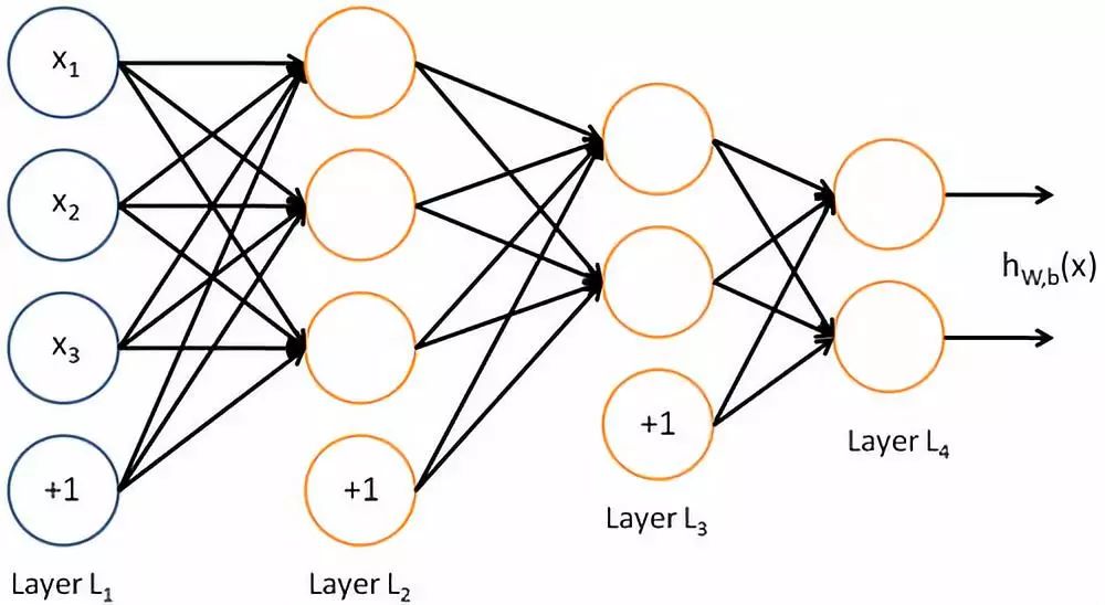
Figure 1
As shown in Figure 1, this is a very simple four-layer neural network, where the leftmost Layer L1 represents the input vector, and the rightmost output vector L4 represents the model’s prediction results for the problem. If applied to the financial business, the leftmost side may represent a user applying for a loan, and the two values in the rightmost vector may represent the probability that this person will default and the probability that this person will repay early in the upcoming repayment period. In the field of text processing, the leftmost side may represent an article, and the two values on the right indicate the probability that this piece of text contains pornographic information; if it is customer review text from e-commerce, it may need to determine the probability of a negative review. The elements at the bottom of layers L1, L2, and L3 represent offsets, which will be discussed later.
As shown in Figure 1, except for Layer L1, each vector value (also called neurons) in the subsequent layers depends on every vector value from the previous layer to perform calculations (in this simplest example, each neuron in every layer depends on all neurons from the previous layer, as indicated by the arrows in the figure. This model is also called a fully connected model. In modern deep learning industrial applications, due to computational load, this form is generally not adopted; instead, selective connections between certain elements are made to reduce computation).
For each unknown neuron in Figure 1, how is the calculation performed? As shown in Figure 2:
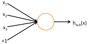
Figure 2
So how is the calculation done? It relies on the choice of the activation function, where the input of this function is a vector and the output is a double value. Here are two commonly used activation functions:

Figure 3(a)
Figure 3(b)
Where exp(-z) is the exponential function and tanh(z) is the hyperbolic tangent function, z=w1x1+w2x2+w3*x3+b, where b is the offset mentioned in figure 1. It can be seen that if there is no b, when the input vector is 0, regardless of how the parameter vector in the activation function (i.e., the vector [w1,w2,w3]) changes, z will always be 0, which is usually not realistic.
Figure 3(a) shows one of the most commonly used activation functions, also known as the sigmoid function. Its range is between 0 and 1. In fact, the input-output mapping of this single “neuron” is essentially a logistic regression (for logistic regression refer to: https://tech.meituan.com/intro_to_logistic_regression.html).
As described above, in this simple model shown in Figure 1, the goal is to ultimately determine the values of the parameter vectors in the seven activation functions. Once a new vector (which could be a loan applicant or an article) arrives, we can use these activation functions to compute the values of each neuron in L2, L3, and L4 (i.e., the seven unknown circles in the figure). After calculating the values of the two neurons in L4, we obtain the final prediction results.
The code snippet for the above steps is as follows:
public double[] predict(double[] x) {
        for (int i = 0; i < x.length; i++) {
            _temp_A[0][i] = x[i];
        }
        predictForwardPass();
        return Arrays.copyOf(_temp_A[layerNum - 1], activationLayerNum[activationLayerNum.length - 1]);
    }

    private void predictForwardPass() {
        for (int l = 1; l < layerNum; l++) {
            for (int i = 0; i < activationLayerNum[l]; i++) {
                _temp_Z[l][i] = innerProduct(_temp_A[l - 1], _W[l - 1][i]) + _B[l - 1];
                _temp_A[l][i] = sigmoid(_temp_Z[l][i]);
            }
        }
    }

    private static double innerProduct(double[] a, double[] b) {
        double sum = 0.0;
        for (int i = 0; i < a.length; i++) {
            sum += (a[i] * b[i]);
        }
        return sum;
    }

    private static double sigmoid(double z) {
        return 1.0 / (1.0 + Math.exp(-z));
    }
So how are the parameters in these seven activation functions determined? This leads us to the core part of model solving, which we will provide a detailed answer to in the next part.