
Selected from arXiv
Compiled by Machine Heart
Contributors: Jiang Siyuan, Smith, Li Yazhou
Recently, a paper titled “Self-Normalizing Neural Networks” published on arXiv has garnered significant attention in the community. It introduces the Scaled Exponential Linear Unit (SELU), which brings in a self-normalizing property. This unit mainly uses a function g to map the mean and variance of two layers of neural networks to achieve normalization. The author of the paper is Sepp Hochreiter, a prominent figure who invented LSTM with Jürgen Schmidhuber, and the previous ELU also came from their group. Interestingly, this NIPS paper, although only 9 pages of main text, has 93 pages of proof in the appendix as shown in the image below.
In this article, Machine Heart provides a summary of the paper. Additionally, there are already comparisons of SELUs with ReLU and Leaky ReLU available on GitHub, which we also introduce.
Paper link: https://arxiv.org/pdf/1706.02515.pdf
Abstract: Deep learning has revolutionized computer vision through Convolutional Neural Networks (CNNs) and transformed natural language processing through Recurrent Neural Networks (RNNs). However, there are few successful cases of deep learning with standard Feedforward Neural Networks (FNNs). Typically, well-performing FNNs are merely shallow models, which cannot mine multi-layered abstract representations. Therefore, we hope to introduce Self-Normalizing Neural Networks (SNNs) to help uncover high-level abstract representations. While batch normalization requires precise normalization, the neuron activation values of SNN can automatically converge to zero mean and unit variance. The activation function of SNN is called the “Scaled Exponential Linear Units (SELUs)”, which introduces the self-normalizing property. By using Banach’s fixed-point theorem, we prove that the activation values approach zero mean and unit variance, and that through many layers of forward propagation, they will still converge to zero mean and unit variance, even in the presence of noise and disturbances. This SNN convergence property allows (1) training of many layers of deep neural networks, (2) strong regularization, and (3) making learning more robust. Furthermore, for activation values that do not approach unit variance, we prove that their variance has upper and lower bounds, thus gradient vanishing and gradient explosion cannot occur. We also took (a) 121 tasks from the UCI Machine Learning repository and compared their performance on (b) new drug discovery benchmarks and (c) astronomical tasks using standard FNNs and other machine learning methods (such as Random Forests, Support Vector Machines, etc.). SNN significantly outperformed all competing FNN methods on the 121 UCI tasks and surpassed all competing methods on the Tox21 dataset, while achieving new records on astronomical datasets. The implemented SNN architecture is generally deeper, and the implementation can be found at the following link: http://github.com/bioinf-jku/SNNs.
Introduction
Deep learning has achieved new records across many different benchmarks and facilitated the development of various commercial applications [25, 33]. Recurrent Neural Networks (RNNs) [18] have brought speech and natural language processing to a new stage. In contrast, Convolutional Neural Networks (CNNs) [24] have transformed computer vision and video tasks.
However, when we review Kaggle competitions, there are usually very few tasks related to computer vision or sequential tasks, and gradient boosting, Random Forests, or Support Vector Machines (SVMs) often achieve excellent performance on the vast majority of tasks. In contrast, deep learning does not perform well.
To train deep Convolutional Neural Networks (CNNs) more robustly, batch normalization has become the standard method for normalizing neuron activation values to have 0 mean and unit variance [20]. Layer normalization [2] ensures 0 mean and unit variance, as if the activation values of the previous layer have 0 mean and unit variance, then weight normalization [32] ensures 0 mean and unit variance. However, normalization techniques are often disturbed during training by stochastic gradient descent (SGD), stochastic regularization (such as dropout), and estimation of normalization parameters.
Self-Normalizing Neural Networks (SNN) are robust to disturbances, and they do not exhibit high variance in training error (see Figure 1). SNN allows neuron activation values to reach 0 mean and unit variance, thus achieving a similar effect to batch normalization, while this normalization effect can maintain robustness across many layers of training. SNN introduces the self-normalizing property based on Scaled Exponential Linear Units (SELU), thus variance stabilization avoids gradient explosion and gradient vanishing.
Self-Normalizing Neural Networks (SNN)
Normalization and SNN
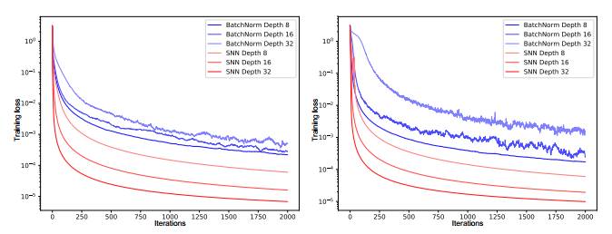
Figure 1: The y-axis of the left and right graphs shows the training loss of Feedforward Neural Networks (FNN) with batch normalization (BatchNorm) and self-normalization (SNN), while the x-axis represents the number of iterations. The neural networks we tested had 8, 16, and 32 layers, with a learning rate of 1e-5. The FNN with batch normalization exhibited larger variance due to disturbances, but SNN did not exhibit large variance, making it more robust to disturbances and speeding up the learning process.
Building Self-Normalizing Neural Networks
We build self-normalizing neural networks by adjusting the properties of function g. Function g has only two design choices: (1) activation function and (2) weight initialization.
Deriving Mean and Variance Through Mapping Function g
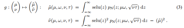
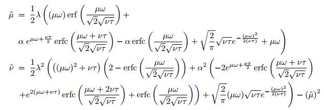
We assume that xi are independent and have the same mean µ and variance ν; of course, the independence assumption is usually not satisfied. We will describe the independence assumption in detail later. Function g maps the mean and variance of the previous layer’s neural network activation values to the mean µ˜ = E(y) and variance ν˜ = Var(y) of the next layer’s activation values y:
The analytical solutions of these integrals can be obtained through the following equations:
Stability of Normalized Weights and Attracting Fixed Point (0, 1)
Stability of Non-Normalized Weights and Attracting Fixed Point
In learning, the normalized weight vector w does not guarantee stability.
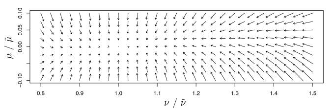
Figure 2: For ω = 0 and τ = 1, the upper graph describes the mapping of mean µ (x-axis) and variance v (y-axis) to the next layer’s mean µ˜ and variance ν˜. The arrows show the direction of the mapping of (µ, ν) by g: (µ, ν) → (˜µ, ν˜). The fixed point of mapping g is (0, 1).
Theorem 1 (Stability and Attracting Fixed Point)
This section gives an outline of the proof of the theorem (detailed proof can be found in Appendix Section A3). According to Banach’s fixed-point theorem, we prove the existence of a unique attracting and stable fixed point.
Theorem 2 (Reducing v)
The detailed proof of this theorem can be found in Appendix Section A3. Therefore, when the mapping passes through many layers, the variance in the interval [3, 16] is mapped to a value less than 3.
Theorem 3 (Increasing v)
The proof of this theorem can be found in Appendix Section A3. All fixed points of the mapping g (Eq. (3)) ensure that 0.8 ≤ τ implies ν ˜ > 0.16, and 0.9 ≤ τ implies ν ˜ > 0.24.
Initialization
Because SNN has fixed points of normalized weights with 0 mean and unit variance, we initialize SNN to meet some expected constraints.
New Dropout Technique
Standard dropout randomly sets an activation value x to 0 with a probability of 1-q, where 0 < q < 1. To maintain the mean, the activation value is scaled by 1/q during training.
Applicability of Central Limit Theorem and Independence Assumption
In the derivative of the mapping (Eq. (3)), we use the Central Limit Theorem (CLT) to approximate the inputs of the neural network  as normally distributed.
Experiments (Omitted)
Conclusion
We have proposed Self-Normalizing Neural Networks and have proven that when neuron activations propagate through the network, they trend toward zero mean and unit variance. Moreover, for activations that do not approach unit variance, we have also proven the upper and lower bounds of variance mapping. Thus, SNN will not produce gradient vanishing and gradient explosion issues. Therefore, SNN is highly suitable for multi-layer structures, allowing us to introduce a brand new regularization mechanism for more robust learning. On the 121 UCI benchmark datasets, SNN has surpassed several other FNNs, including those with or without normalization methods, such as batch normalization, layer normalization, weight normalization, or other special structures (Highway network or Residual network). SNN has also yielded perfect results in drug discovery and astronomical tasks. Compared to other FNN networks, high-performance SNN structures are usually deeper.
Appendix (Omitted)
Comparison of SELU with Relu and Leaky Relu
Yesterday, Shao-Hua Sun released a comparison of SELU with Relu and Leaky Relu on GitHub, and Machine Heart translated and introduced the comparison results. The specific implementation process can be found at the following project address.
Project address: https://github.com/shaohua0116/Activation-Visualization-Histogram
Description
This experiment includes the TensorFlow implementation of SELUs (Scaled Exponential Linear Units) proposed in the paper “Self-Normalizing Neural Networks”. It also aims to compare SELUs, ReLU, and Leaky-ReLU. The focus of this experiment is to visualize activations on TensorBoard.
Visualization and histogram comparison of SELUs (Scaled Exponential Linear Units), ReLU, and Leaky-ReLU
Theoretically, we hope that the mean of activations in each layer is 0 (zero mean) and the variance is 1 (unit variance) to ensure that the tensors propagating between layers converge (mean of 0, variance of 1). This avoids sudden gradient vanishing or explosive growth, thus stabilizing the learning process. In this experiment, the authors propose SELUs (Scaled Exponential Linear Units) aimed at automatically shifting and rescaling neuron activations to achieve zero mean and unit variance without explicit normalization.
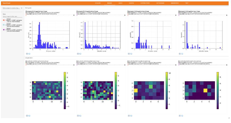
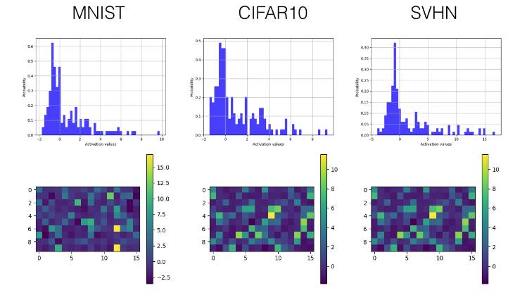
To experimentally demonstrate the effectiveness of the proposed activations, a convolutional neural network with three convolutional layers (also including three fully connected layers) was trained on the MNIST, SVHN, and CIFAR10 datasets for image classification. To overcome some limitations of TensorBoard display, we introduced the plotting library TensorFlow Plot to bridge the gap between Python plotting libraries and TensorBoard. Here are some examples.
-
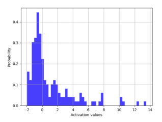
Histogram of activation values on TensorBoard
-
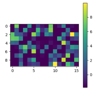
Visualization of activation values on TensorBoard
Training and testing of the implemented model on three public datasets: MNIST, SVHN, and CIFAR-10.
Results
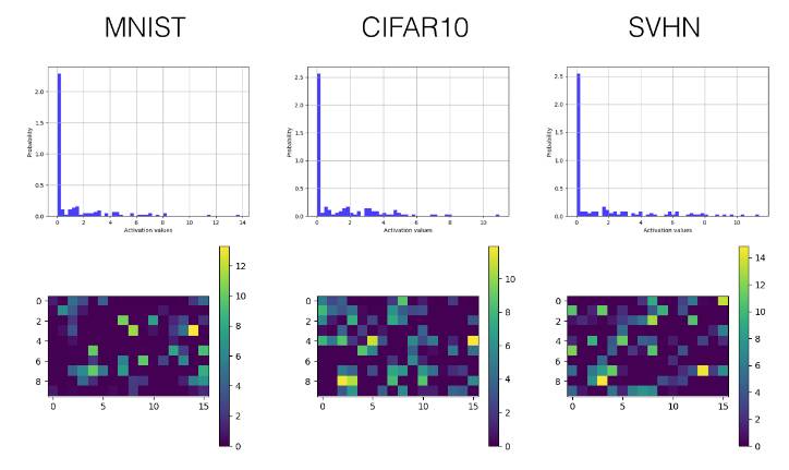
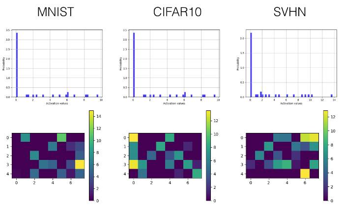
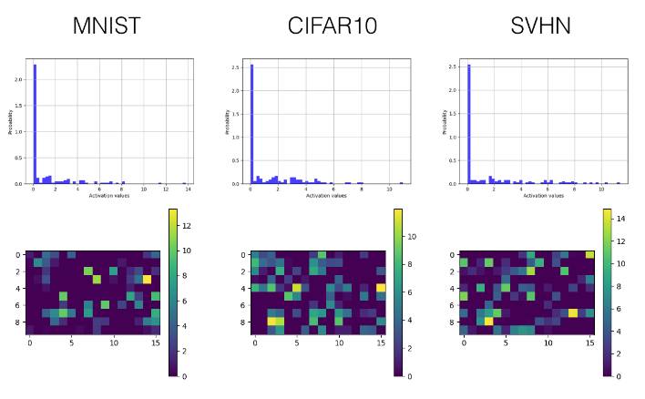
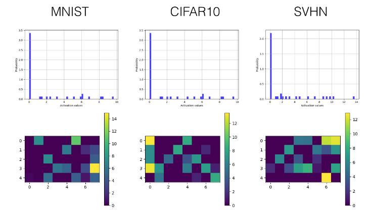
Below, we selectively display the histograms and visualized activation value graphs of the last convolutional layer (the third layer) and the first fully connected layer (the fourth layer).
SELU
-
Convolutional Layer
-
Fully Connected Layer
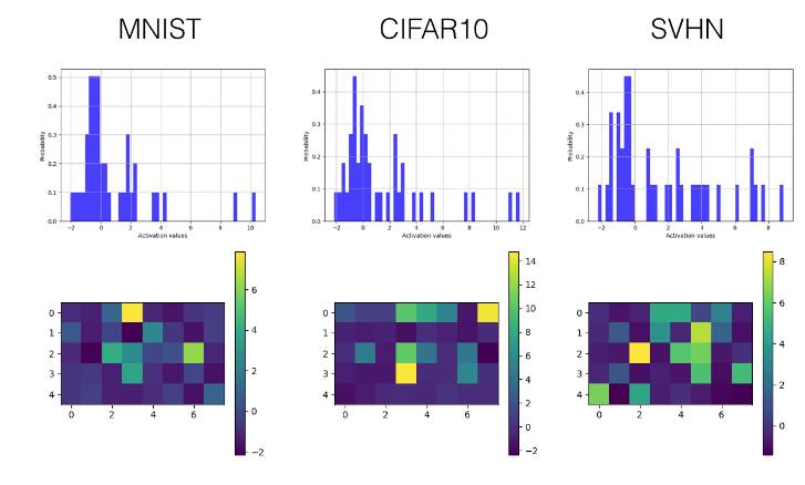
ReLU
-
Convolutional Layer
-
Fully Connected Layer
Leaky ReLU
-
Convolutional Layer
-
Fully Connected Layer
Related Work
-
Self-Normalizing Neural Networks by Klambauer et al.
-
Rectified Linear Units Improve Restricted Boltzmann Machines by Nair et al.
-
Empirical Evaluation of Rectified Activations in Convolutional Network by Xu et al.
Authors
-
Shao-Hua Sun / @shaohua0116 (https://shaohua0116.github.io/).

This article is compiled by Machine Heart, please contact this public account for authorization to reprint.
✄————————————————
Join Machine Heart (Full-time Reporter/Intern): [email protected]
Submissions or Seeking Coverage: [email protected]
Advertising & Business Cooperation: [email protected]
Click to read the original text and visit the Machine Heart official website↓↓↓