
When I first started exploring machine learning algorithms, I was overwhelmed by all the mathematical content. I found that without fully understanding the intuition behind the algorithm, it was difficult to grasp the underlying mathematical principles. Therefore, I tend to favor explanations that break down the algorithm into simpler, more digestible steps. This is what I am attempting to do today: explain the XGBoost algorithm in a way that even a 10-year-old can understand. Let’s get started!
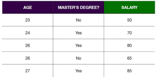
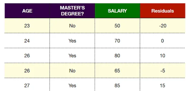
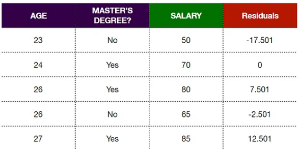
Let’s start with a training dataset that contains 5 samples. Each sample records their age (AGE), whether they have a master’s degree (MASTER’S DEGREE), and their salary (SALARY) (in thousands), with the goal of using the XGBoost model to predict salary.
Step 1: Make an Initial Prediction and Calculate Residuals
This prediction can be any value. But let’s assume the initial prediction is the average of the variable we want to predict.
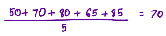
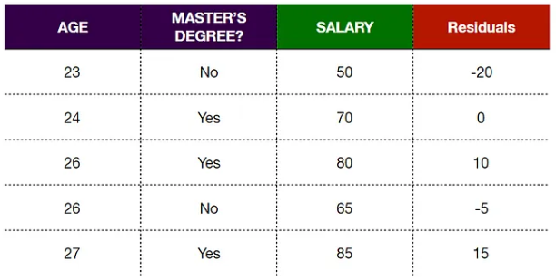
We calculate the residuals using the following formula:
Here, our observed values are the values in the Salary column, and all predicted values are equal to 70 (the initial prediction).
The residual values for each sample are as follows:
Step 2: Build the XGBoost Decision Tree
Each tree starts from a root node, and all residuals enter that root node.

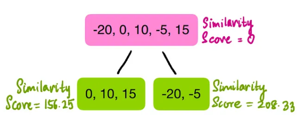
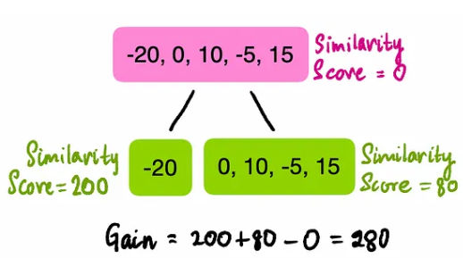
Now we need to calculate the similarity score for that root node.
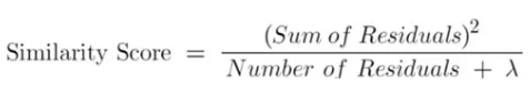
Where the Sum of Residuals means the sum of the residuals, the Number of Residuals means the count of residuals, and λ (lambda) is a regularization parameter that reduces the sensitivity of predictions to individual observations and prevents overfitting (i.e., the model fitting perfectly to the training dataset). The default value of λ is 1, so in this example, we set λ = 1.

Now we should see if we can better cluster the residuals by splitting them into two groups based on the predictive variables (age and master’s degree). Splitting the residuals means adding branches to the tree.
First, let’s try to split this leaf using “Do they have a master’s degree?”

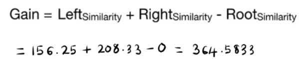
Then calculate the similarity scores for the left and right leaf nodes after the split:
Now, by splitting the residuals based on “Do they have a master’s degree,” we compare the similarity before and after the split. Define Gain as the difference between the similarity after the split and the similarity before the split; if the gain is positive, then the split is a good idea; otherwise, it is not. The gain calculation:
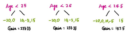
Then we compare this gain with the gain from splitting by age. Since age is a continuous variable, the process of finding different splits is somewhat complex. First, we sort the rows of the dataset in ascending order by age and then calculate the average of adjacent age values.
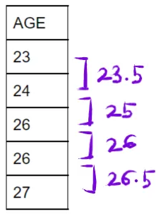
Now we use these four averages as thresholds to split the residuals and calculate the gain for each split. The first split uses age < 23.5.
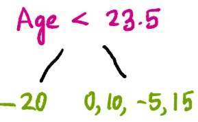
For this split, we calculate the similarity scores and gain in a manner similar to that for the master’s degree.
Then we calculate the remaining age splits in the same manner:
Among all the master’s degree splits and the four age splits, the split based on “Do they have a master’s degree” has the highest gain value, so we will use it as our initial split. Now we can split our master’s degree leaf into more branches by again using the same process described above. But this time, we will use the initial master’s degree leaf as the root node and try to split it by achieving a maximum gain greater than 0.
Let’s start with the left node. For this node, we only consider the observations where the value in the master’s degree column is “Yes,” as only these observations will fall into the left node.

Thus, we use the same process to calculate the gain for age splits, but this time only using the residuals from the highlighted rows in the image above.
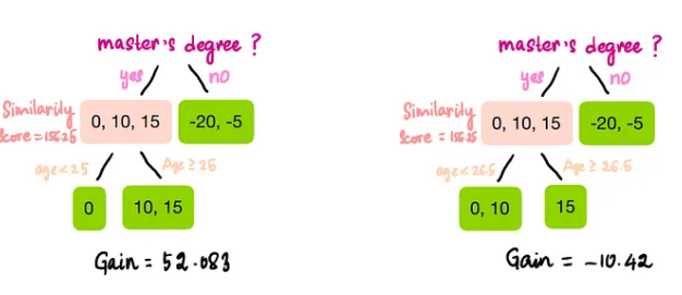
Since only age < 25 gives us a positive gain, we use this threshold to split the left node.
Next, we turn to the right node, where the master’s degree value is “No.” We will only calculate the residuals from the highlighted rows in the image below.
In the right node, we only have two observations, so the only possible split is age < 24.5, as this is the average of the two age values (23 and 26) in the highlighted rows.
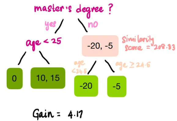
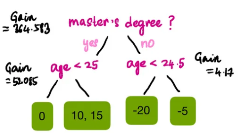
The gain for this split is positive, so our final tree is:

Step 3: Tree Pruning
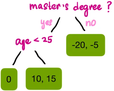
Tree pruning is another method we use to avoid overfitting the data. To do this, we start from the bottom of the tree and gradually move up to check whether the splits are valid. To determine validity, we use γ (gamma). If the gain minus γ is positive, we keep that split; otherwise, we remove it. The default value of γ is 0, but for illustration purposes, let’s set γ to 50. Based on previous calculations, we know the gain values for all nodes:
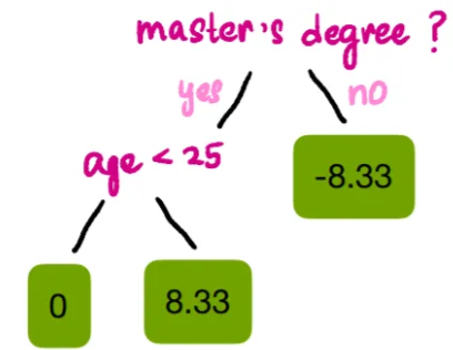
Since all splits except the one for age < 24.5 have gains greater than γ, we can remove that branch. Thus, the final tree structure is:
Step 4: Calculate Values for Leaf Nodes
Since leaf nodes cannot provide multiple outputs, we need to calculate the output based on the sample values contained in the leaf nodes.
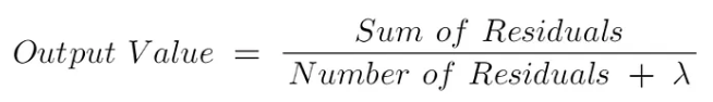
Where the Sum of Residuals means the sum of the residuals, and the Number of Residuals means the count of residuals.
The calculation of the output value for leaf nodes is similar to the similarity score, but we do not square the residuals. Using this formula and λ = 1, we obtain the output values for all leaf nodes:
Step 5: Model Prediction
Now that all the hard work of building the model is done, we come to the exciting part: seeing how our new model improves our predictions. We can use the following formula to make predictions.
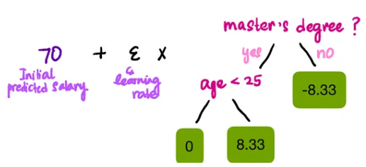
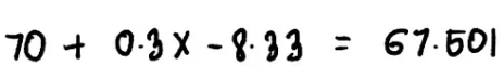
As shown in the figure, 70 is the model’s initial prediction, which is the learning rate, set to 0.3 in this article.
Thus, the predicted value for the first observation is 67.501.
Similarly, we can calculate the predicted values for other observations:
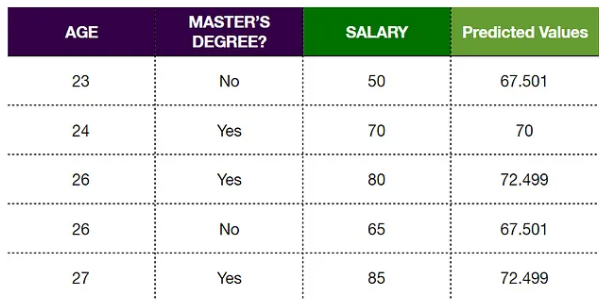
Step 6: Calculate Residuals for New Predictions
We find that the new residuals are smaller than before, indicating that we have taken a small step in the right direction. As we repeat this process, our residuals will get smaller and smaller, indicating that our predicted values are getting closer to the observed values.
Step 7: Repeat Steps 2-6
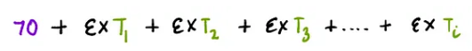
Now we just need to repeat this process over and over: build a new tree, make predictions, and calculate residuals in each iteration. We will repeat this process until the residuals become very small or we reach the maximum iterations set for the algorithm. If the trees built in each iteration are represented, where i is the current iteration number, then the formula for calculating predictions is:
That’s it! Thank you for reading, and I wish you all the best on your upcoming journey with algorithms!
Feel free to scan the code to follow: