
Source | British Wenwen Education
Author | Yichen
The empirical graduation thesis in finance and economics mainly consists of time series and panel data. As July approaches, many students have started working on the data analysis part of their theses. But how to operate Eviews for time series model analysis? Wenwen is fortunate to have invited Dr. Yichen from Newcastle University to present this Eviews operation guide, providing some relief for those struggling with Eviews data analysis in the hot summer.
Time Series and Panel Data
Before sharing the Eviews operations, let’s first distinguish between time series and panel data to help those writing their theses clarify whether they are conducting time series or panel data analysis.
Time series: Data collected at different points in time, primarily reflecting the changes in a certain phenomenon over time.
For example: The GDP of country A for the years 2015, 2016, 2017, 2018, and 2019 is 8, 9, 10, 11, 12 respectively.
Panel data: Contains both time series and cross-sectional dimensions, arranged on a plane, which is significantly different from data that is arranged in a single dimension, resembling a panel.
For example: The GDP of various countries for the years 2015, 2016, 2017, 2018, and 2019 is as follows:
Country A: 8, 9, 10, 11, 12;
Country B: 9, 10, 11, 12, 13;
Country C: 5, 6, 7, 8, 9;
Country D: 7, 8, 9, 10, 11.
In simple terms: Time series mainly considers the time dimension, while panel data needs to consider both time and space dimensions.
Eviews Software Introduction
Eviews stands for Econometrics Views, commonly referred to as an econometric software package. In empirical finance and economics theses, econometrics is inevitably used, and we apply econometric methods to design models, collect data, estimate models, test models, and apply models (structural analysis, economic forecasting, policy significance evaluation) to better observe the quantitative laws of socio-economic relationships and economic activities. In time series analysis, Eviews, with its simple and visual operation style, has become the choice for beginners. Even in complex models, Eviews is often used in conjunction with Matlab and Gauss to analyze the basic characteristics of data.
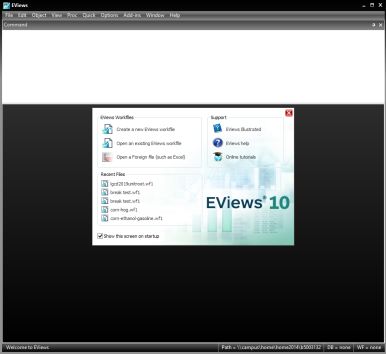
▲ Figure 1. Eviews Main Interface
Unit Root Test
Since time series data spans a long time period, using the unit root test to determine whether the data is stationary is the first operation that must be performed for any model (VAR, Granger Causality, Cointegration, or VECM). This is the essential first step.
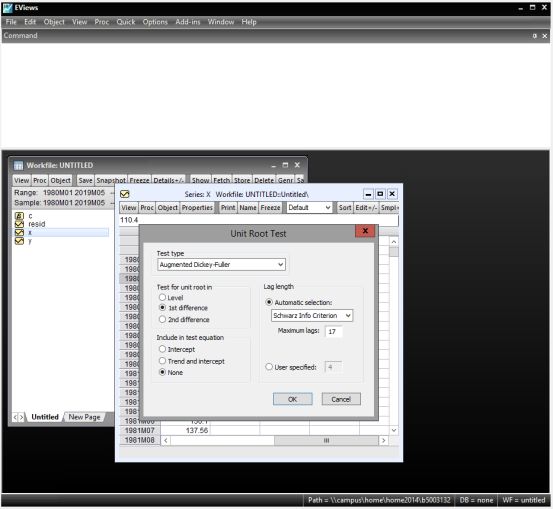
Step 1: After inputting the data, we want to test the stationarity of the independent variable x. Double-click x to open the dialog box shown in Figure 1, select View — Unit Root Test, and in the pop-up dialog, select Augmented Dickey-Fuller – Level and choose Intercept or Trend or Both (based on the linear graph of the data to determine whether there is an intercept or trend). In Automatic Selection, choose Akaike Info Criterion (AIC) or Schwarz Info Criterion (SIC). After confirming, we obtain the results and use the P-value to determine whether to reject the null hypothesis of the existence of a unit root (Figure 2).

▲ Unit Root Test Step 1
Step 2: After obtaining the results, double-click x again to open the dialog box shown in Figure 1. This time select View — Unit Root Test, and in the pop-up dialog, select Augmented Dickey-Fuller – 1st difference – none. In Automatic Selection, choose AIC or SIC. After confirming, we obtain the results and use the P-value to determine whether to reject the null hypothesis of the existence of a unit root (Figure 3).
▲ Unit Root Test Step 2
Step 3: After performing Step 1 and not rejecting the null hypothesis, but rejecting it after Step 2, we say that the data has a unit root, being I(1). If we can reject the null hypothesis after Step 1, the data is stationary, I(0).
VAR Model
Establishing a VAR model involves five processes:
(1) Establish VAR and determine lag order
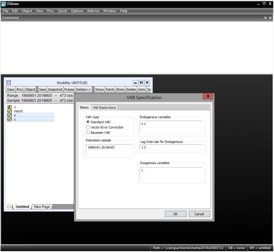
Step 1: After inputting the data, select both x and y, right-click, and choose Open — as VAR. In the pop-up dialog, select Standard VAR, input y and x in Endogenous Variables, and choose any value in Lag Intervals for Endogenous Variables (we choose the default of 1 2). In Exogenous Variables, input c and click confirm (Figure 4).
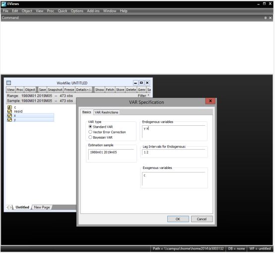
▲ VAR Model Step 1
Step 2: In the preliminary established VAR menu, select View — Lag Structure — Lag Length Criteria. In the pop-up dialog, input 10 or more (Figure 5). The result with the most asterisks will be the optimal lag order. For example, if it is 3, then it is VAR(3) (Figure 6).
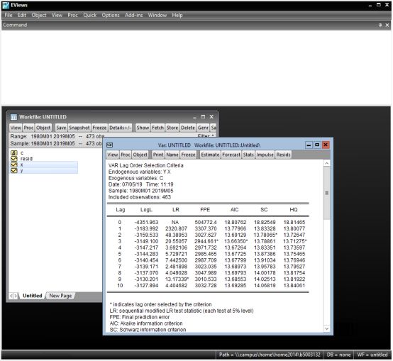
▲ VAR Model Step 2
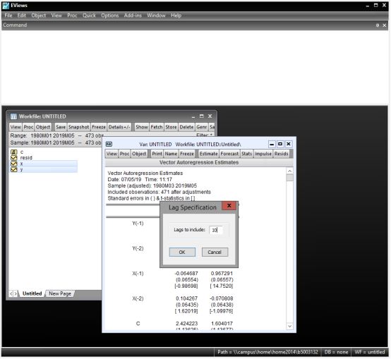
▲ VAR Model Step 2
Step 3: Repeat Step 1, keeping other inputs unchanged, and in Lag Intervals, input the optimal lag order with the most asterisks. For example, input 3 to establish the VAR(3) model and obtain the regression results (Figure 7).
▲VAR Model Step 3
(2) Testing for Exogeneity of Variables
In the established VAR menu, select View — Lag Structure — Granger causality/Block exogeneity tests
(3) Model Stability Assessment
In the established VAR menu, select View — Lag Structure — AR Roots Table. If the absolute values of the numbers obtained are all less than 1, then the VAR is stable.
(4) Impulse Response
In the established VAR menu, directly select Impulse. In the pop-up dialog, select Multiple Graphs to obtain multiple graphs (Figure 8).
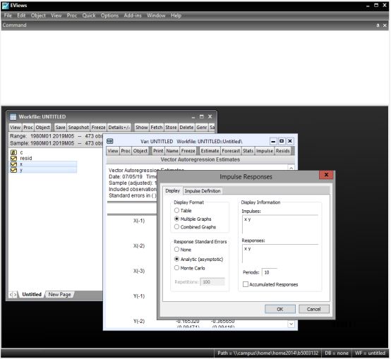
▲Impulse Response
(5) Variance Analysis
In the established VAR menu, select View — Variance Decomposition. In the pop-up dialog, input the variables for variance decomposition, which can be one or multiple (Figure 9).
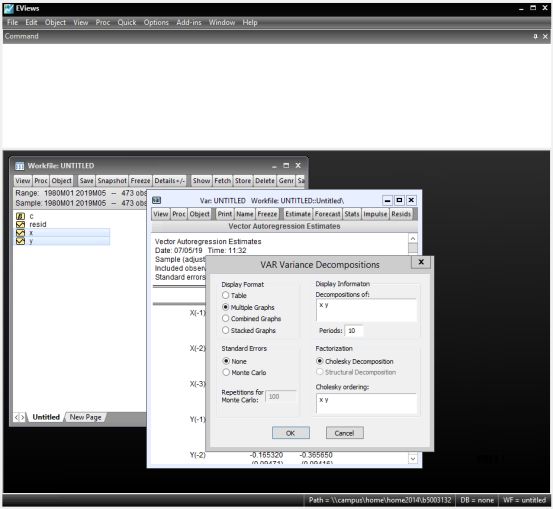
▲ Variance Analysis
Granger Causality Test
Select both x and y after inputting the data, right-click, and choose Open — as Group — View — Granger Causality
Engle-Granger Cointegration Test
In the latest version of Eviews, we can use a straightforward method to test for single or multiple cointegration relationships without the complex two-step method.
Select both x and y after inputting the data, right-click, and choose Open — as Group — View — Cointegration Test — Single Equation Cointegration Test. In the pop-up dialog, select Engle-Granger from the method dropdown. In the Trend Specification dropdown, choose whether there is an intercept or trend based on the data performance. In the Lag Specification dropdown, select AIC or SIC (note: if AIC was chosen in the unit root test, AIC must also be selected here for consistency). The results can directly use the tau-statistic corresponding to the P-value to determine whether to reject the null hypothesis of no cointegration relationship (Figure 10).
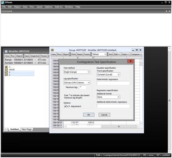
▲ Figure 10. Engle-Granger Cointegration Test
Johansen Cointegration Test
The Johansen cointegration test is conducted based on the established VAR model, and the testing process includes:
(1) Unit Root Test
(2) Establish VAR and determine lag order
(3) Johansen Cointegration Test
For processes (1) and (2), refer to the VAR model operation steps above. Here, we mainly introduce the operational settings for the Johansen cointegration test.
In the established VAR menu, select View — Cointegration Test. The pop-up dialog includes five different scenarios for cointegration testing, which can be selected based on personal data performance. All five can also be selected to compare results. In Lag intervals, input a lag order one less than that in the VAR model, and confirm (Figure 11).

▲ Figure 11. Johansen Cointegration Test
VECM Model
The cointegration test is primarily used to study the long-term relationships between variables, while the VECM model is used to analyze how short-term deviations from equilibrium are adjusted back to equilibrium. Therefore, VECM operations are conducted after the Johansen test.
In the established VAR menu, select Estimate — Basics — VAR type – Vector Error Correction. Here, it is important to note that in the Lag Intervals for D box, input a lag order one less than that set in the VAR (Figure 12). Click on Cointegration – Rank next to Basics, and set the Number of Cointegrating based on the number provided by the Johansen cointegration test, selecting one of the five options based on data performance (Figure 13).
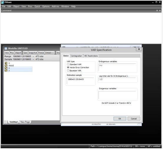
▲ Figure 12. VECM Model
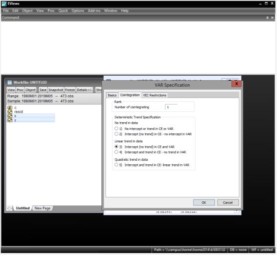
▲ Figure 13. VECM Model
Several very important time series model operation processes have been sincerely presented!
Providing some relief for those struggling with Eviews data analysis in the hot summer.
Wishing everyone success in defeating data analysis!
Entering the writing-up stage!
Guest Speaker:

Yichen
2016-Present, PhD in Economics at Newcastle University
2015-2016, Master’s in Banking and Finance at Newcastle University