


1. ANSYS and Structural Analysis

 ANSYS software is a large general-purpose finite element analysis software that integrates structural, fluid, electromagnetic, acoustic, and thermal field analysis, widely used in civil, geological, mining, materials, mechanical, and hydraulic engineering analysis and research. It can run on most computers and operating systems (such as Windows, UNIX, Linux, HP-UX, etc.) and can interface with most CAD software.Structural analysis is used to determine the deformation, strain, stress, and reaction forces of structures. It includes the following types:Static analysis – used for static loads. It can consider both linear and nonlinear behavior of structures, such as large deformations, large strains, stress stiffening, contact, plasticity, hyperelasticity, and creep.Buckling analysis – used to calculate linear buckling loads and determine buckling mode shapes. Nonlinear buckling analysis can also be performed.Modal analysis – calculates the natural frequencies and mode shapes of linear structures.Harmonic response analysis – determines the response of linear structures to loads that vary sinusoidally over time.Transient dynamic analysis – determines the response of structures to loads that vary arbitrarily over time. It can consider the same nonlinear behaviors as static analysis.Spectral analysis – an extension of modal analysis, used to calculate stresses and strains in structures caused by random vibrations (also called response spectrum or PSD).Explicit dynamic analysis – ANSYS/LS-DYNA (explicit dynamic analysis module) can be used to compute highly nonlinear dynamic problems and complex contact issues.Specialized analysis – fracture analysis, composite material analysis, fatigue analysis.


2. The three main steps in the ANSYS analysis process:

 1. Create Finite Element Model – Create or import geometric models. – Define material properties. – Mesh elements (nodes and elements).2. Apply Loads and Solve – Apply loads and load options. – Solve.3. View Results – View analysis results. – Verify results. (Check if the analysis is correct)


3. Geometric Modeling

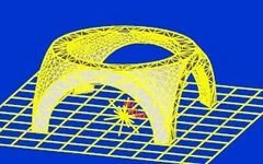
 Geometric modeling in ANSYS typically includes two methods: bottom-up modeling and top-down modeling.Bottom-up modeling, as the name suggests, constructs a solid model from the lowest unit of the model to the highest unit. This means defining key points first and then using these key points to define higher-level solid elements, such as lines, surfaces, and solids.ANSYS allows modeling by assembling geometric voxels such as lines, surfaces, and solids. When a voxel is generated, the ANSYS program automatically generates all lower-level elements belonging to that voxel. This method of constructing a model from higher-level solid elements is known as top-down modeling.Geometric modeling GUI path: Main Menu -> Preprocessor -> Modeling -> CreateBoolean operations refer to the combination calculations of geometric elements. ANSYS’s Boolean operations include add, subtract, intersect, divide, glue, and overlap. They apply not only to simple elements within voxels but also to complex geometric models imported from CAD systems.
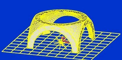 This seemingly complex model is actually the result of an intersection Boolean operation between a cube and a hollow sphere.Boolean operation GUI path: Main Menu -> Preprocessor -> Modeling -> Operate


4. Element Properties

 To define element properties, it is first necessary to establish some element property tables. Typical properties include element type (GUI path: Main Menu -> Preprocessor -> Element Type -> ADD/EDIT/DELETE), real constants (GUI path: Main Menu -> Preprocessor -> Real constants), and material properties (Main Menu -> Preprocessor -> Material Props -> Material option).
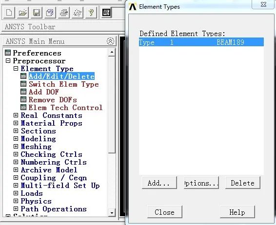 Establishing element types
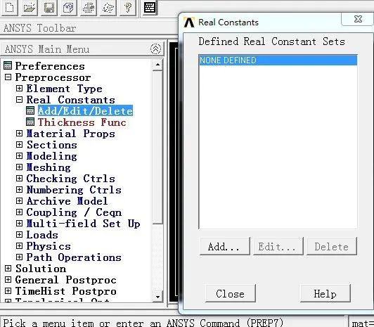 Establishing real constants
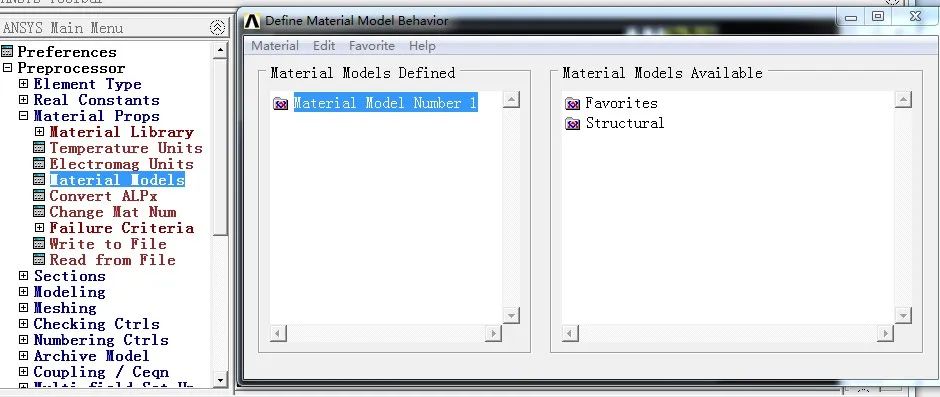 Establishing material properties


5. Mesh Generation

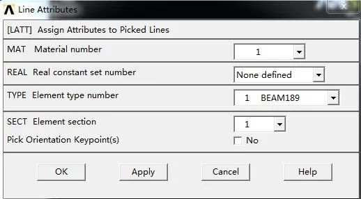
 1. Define Element PropertiesOnce the element property table is established, element properties can be assigned to different parts of the model by referencing the appropriate entries in the table. The references are sets of identification numbers, including material number (MAT), real constant number (TEAL), element type number (TYPE), coordinate system number (ESYS), etc. Element properties can be directly assigned to the selected solid model elements.GUI path: Main Menu -> Preprocessor -> Meshing -> Mesh Attributes, defining points, lines, surfaces, or solids based on the geometric model.
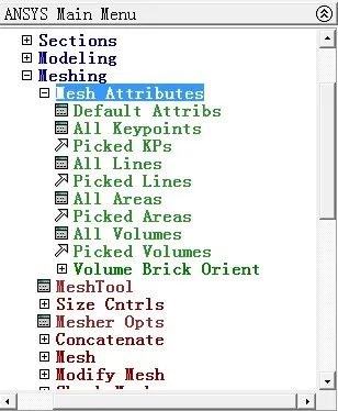
 Defining element properties2. Perform Mesh GenerationANSYS can use mesh generation tools to achieve quick meshing (GUI path Main Menu -> Preprocessor -> Meshing -> Mesh tool)This mesh generation tool includes the following functions:1. Element property control2. Intelligent mesh generation control3. Size control4. Specify element shape
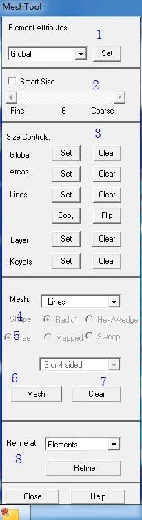 5. Free mesh generation or mapped mesh generation6. Execute mesh generation7. Clear mesh8. Local refinementAfter selecting the options, click Mesh, select the geometric model to be meshed, and click OK to obtain its finite element model.
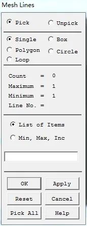


6. Loading and Solving

 1. LoadingThe primary purpose of finite element analysis is to examine the response of structures or components under certain loading conditions. Therefore, analyzing appropriate loading conditions is a critical step.In ANSYS, loads can be categorized as:Degrees of freedom (DOF) – defining the values of the degrees of freedom (DOF) at nodes (structural analysis – displacement, thermal analysis – temperature, electromagnetic analysis – magnetic potential, etc.)Concentrated loads – point loads (structural analysis – force, thermal analysis – thermal conductivity, electromagnetic analysis – magnetic current segments)Surface loads – distributed loads acting on surfaces (structural analysis – pressure, thermal analysis – thermal convection, electromagnetic analysis – magnetic Maxwell surfaces, etc.)Volume loads – acting within a volume or field (thermal analysis – volumetric expansion, internal heat generation, electromagnetic analysis – magnetic current density, etc.)Inertial loads – loads caused by structural mass or inertia (gravity, angular velocity, etc.)In ANSYS software, loads can be applied to both solid models and finite element models.
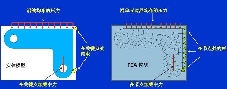 Regardless of the loading method, ANSYS will convert the loads to the finite element model before solving. Therefore, loads applied to solids will automatically convert to their respective nodes or elements.Load application GUI path: Main Menu -> Preprocessor -> Loads -> Apply -> Structural
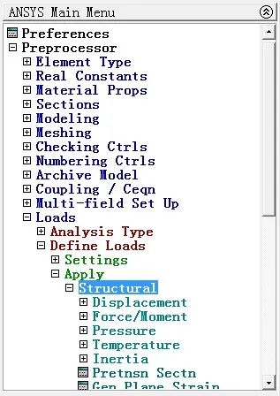 2. SolvingBefore solving, it is necessary to check the analysis data, confirm its accuracy, save the data, and review the solving information.Solve GUI path: Main Menu -> Solution -> Solve -> Current LSAfter that, save the file and view the calculation results in the General PostprocessorGUI path: Main Menu -> General Postprocessor -> Plot Results


7. ANSYS Structural Stability Analysis

 ANSYS software calculates the critical load of structures through buckling analysis, which is a technique used to determine the buckling load and mode shapes of structures. Typically, eigenvalue buckling analysis is used to predict the theoretical buckling strength of ideal elastic structures.For buckling analysis, the static solution of the structure must first be obtained, usually by applying a unit load. However, the maximum eigenvalue allowed by ANSYS is 1,000,000. If the eigenvalue exceeds this limit, a larger load must be applied. When a load is applied, the solved eigenvalue indicates the critical load; when a non-unit load is applied, the solved eigenvalue multiplied by the applied load gives the critical load.(1) Enter the solver Main menu -> Solution(2) Specify analysis type Main menu -> Solution -> Analysis Type -> New Analysis(3) Specify analysis options Main menu -> Solution -> Analysis Type -> Sol’n controls, select Calculate prestress effects and confirm.(4) Solve Main Menu -> Solution -> Solve -> Current LS(5) Exit the solver Main Menu -> FinishAfter obtaining the static solution of the structure, it is necessary to obtain the eigenvalue buckling solution.(1) Enter the solver Main menu -> Solution(2) Specify analysis type Main menu -> Solution -> Analysis Type -> New Analysis(3) Specify analysis options Main menu -> Solution -> Analysis Type -> Analysis Options(4) Solve Main Menu -> Solution -> Solve -> Current LS(5) End Main Menu -> FinishExtended solution:(1) Re-enter the solver Main menu -> Solution(2) Specify extended solution Main menu -> Solution -> Analysis Type -> Expansion Pass(3) Specify extended solution options Main menu -> Solution -> Load Step Opts -> Expansion pass -> Single Modes -> Expand Modes(4) Solve Main Menu -> Solution -> Solve -> Current LS(5) Leave the solver Main Menu -> FinishThe buckling expansion results are written to the structural results file, including buckling load factors, buckling mode shapes, and corresponding stress distributions, which can be observed in the general postprocessor.(1) List buckling load factorsGUI path Main Menu -> General Postproc -> Results Summary(2) Read specified modes to display buckling mode shapes. Each buckling mode is stored in a separate result step.GUI path Main Menu -> General Postproc -> Read Results -> By load Step(3) Display buckling mode shapesGUI path Main Menu -> General Postproc -> Plot Results -> Deformed Shape(4) Display corresponding stress distribution contour plotsGUI path Main Menu -> General Postproc -> Plot Results -> Contour Plot -> Nodal Solution.
Source: Baidu Wenku, Author: Yezipei
2024 Annual Plan Pre-selection
- Method 1: Scan the QR code below with WeChat to enter the page

- Method 2: 18510898133 (WeChat) Manager Li
Feel free to forward
 Share
Share Collect
 Like
Like View
View
| Disclaimer:This public account article includes but is not limited to content that is reprinted or shared. We maintain neutrality regarding its statements and viewpoints. The purpose is solely to convey more information and does not represent this account’s endorsement of its views or verification of its descriptions. All copyrights belong to the original author. Original works have been declared; reprinting requires application and authorization from this account!