Introduction
When constructing models, especially when dealing with the input-output data formats between layers, some commonly used data processing functions such as tensor calculations and broadcasting mechanisms are very important. They remain indispensable when later using the Transformers library with pre-trained models. This article aims to explain the most commonly used Pytorch processing functions for easy reference in the future.
The Transformers library is built on top of the Pytorch framework (the Tensorflow version is not fully functional). Although the official claim is that using the Transformers library does not require mastering Pytorch knowledge, in practice, we still need to use Pytorch’s DataLoader class to load data and use Pytorch’s optimizers to adjust model parameters, etc.
Therefore, this chapter will introduce some basic concepts of Pytorch and classes that may be used later, allowing everyone to quickly get started with using the Transformers and Pytorch libraries to build models.
1. Basics of Pytorch
Pytorch (https://pytorch.org/) was launched by Facebook’s AI Research in 2017, featuring powerful GPU-accelerated tensor computation capabilities and automatic differentiation, allowing model parameters to be optimized using gradient-based methods. As of August 2022, Pytorch has become one of the top 5 fastest-growing open-source communities in the world, alongside the Linux kernel and Kubernetes. Now, over 80% of researchers at top machine learning conferences such as NeurIPS and ICML use Pytorch.
Tensors
A tensor is the foundation of deep learning; for instance, a common 0-dimensional tensor is called a scalar, a 1-dimensional tensor is called a vector, and a 2-dimensional tensor is called a matrix. Essentially, Pytorch is a mathematical computation toolkit based on tensors, providing various ways to create tensors:
>>> import torch
>>> torch.empty(2, 3)  # empty tensor (uninitialized), shape (2,3)
tensor([[2.7508e+23, 4.3546e+27, 7.5571e+31],
        [2.0283e-19, 3.0981e+32, 1.8496e+20]])
>>> torch.rand(2, 3)  # random tensor, each value taken from [0,1)
tensor([[0.8892, 0.2503, 0.2827],
        [0.9474, 0.5373, 0.4672]])
>>> torch.randn(2, 3)  # random tensor, each value taken from standard normal distribution
tensor([[-0.4541, -1.1986,  0.1952],
        [ 0.9518,  1.3268, -0.4778]])
>>> torch.zeros(2, 3, dtype=torch.long)  # long integer zero tensor
tensor([[0, 0, 0],
        [0, 0, 0]])
>>> torch.zeros(2, 3, dtype=torch.double)  # double float zero tensor
tensor([[0., 0., 0.],
        [0., 0., 0.]], dtype=torch.float64)
>>> torch.arange(10)
tensor([0, 1, 2, 3, 4, 5, 6, 7, 8, 9])
Tensors can also be created based on existing arrays or Numpy arrays using torch.tensor() or torch.from_numpy():
>>> array = [[1.0, 3.8, 2.1], [8.6, 4.0, 2.4]]
>>> torch.tensor(array)
tensor([[1.0000, 3.8000, 2.1000],
        [8.6000, 4.0000, 2.4000]])
>>> import numpy as np
>>> array = np.array([[1.0, 3.8, 2.1], [8.6, 4.0, 2.4]])
>>> torch.from_numpy(array)
tensor([[1.0000, 3.8000, 2.1000],
        [8.6000, 4.0000, 2.4000]], dtype=torch.float64)
Note: The tensors created in the above ways will be stored in memory and computed using the CPU. If you want to utilize GPU computation, you need to create tensors directly on the GPU or send them to the GPU:
>>> torch.rand(2, 3).cuda()
tensor([[0.0405, 0.1489, 0.8197],
        [0.9589, 0.0379, 0.5734]], device='cuda:0')
>>> torch.rand(2, 3, device="cuda")
tensor([[0.0405, 0.1489, 0.8197],
        [0.9589, 0.0379, 0.5734]], device='cuda:0')
>>> torch.rand(2, 3).to("cuda")
tensor([[0.9474, 0.7882, 0.3053],
        [0.6759, 0.1196, 0.7484]], device='cuda:0')
In subsequent chapters, we will often send the encoded text tensors to the specified GPU or CPU using to(device).
Tensor Calculations
The addition, subtraction, multiplication, and division of tensors are performed element-wise. For example:
>>> x = torch.tensor([1, 2, 3], dtype=torch.double)
>>> y = torch.tensor([4, 5, 6], dtype=torch.double)
>>> print(x + y)
tensor([5., 7., 9.], dtype=torch.float64)
>>> print(x - y)
tensor([-3., -3., -3.], dtype=torch.float64)
>>> print(x * y)
tensor([ 4., 10., 18.], dtype=torch.float64)
>>> print(x / y)
tensor([0.2500, 0.4000, 0.5000], dtype=torch.float64)
Pytorch also provides many commonly used calculation functions, such as torch.dot() for calculating the dot product of vectors, torch.mm() for matrix multiplication, trigonometric functions, and various mathematical functions:
>>> x.dot(y)
tensor(32., dtype=torch.float64)
>>> x.sin()
tensor([0.8415, 0.9093, 0.1411], dtype=torch.float64)
>>> x.exp()
tensor([ 2.7183,  7.3891, 20.0855], dtype=torch.float64)
In addition to mathematical operations, Pytorch also provides a variety of tensor operation functions, such as aggregation, concatenation, comparison, random sampling, serialization, etc. For detailed usage, please refer to the Pytorch official documentation (https://pytorch.org/tutorials/beginner/basics/tensorqs_tutorial.html).
When performing aggregation operations (such as calculating the average, sum, maximum, and minimum) or concatenation, you can specify the dimension (dim) for the operation. For example, to calculate the average of a tensor, it will calculate the average of all elements by default:
>>> x = torch.tensor([[1, 2, 3], [4, 5, 6]], dtype=torch.double)
>>> x.mean()
tensor(3.5000, dtype=torch.float64)
More commonly, you may need to calculate the average of a specific row or column, in which case you need to set the dimension for the calculation, for example, calculating the averages for dimensions 0 and 1 respectively:
>>> x.mean(dim=0)
tensor([2.5000, 3.5000, 4.5000], dtype=torch.float64)
>>> x.mean(dim=1)
tensor([2., 5.], dtype=torch.float64)
Note that the above calculations automatically remove extra dimensions, so the result changes from a matrix to a vector. If you want to retain the dimensions, you can set keepdim=True:
>>> x.mean(dim=0, keepdim=True)
tensor([[2.5000, 3.5000, 4.5000]], dtype=torch.float64)
>>> x.mean(dim=1, keepdim=True)
tensor([[2.],
        [5.]], dtype=torch.float64)
The concatenation operation torch.cat works similarly; by specifying the concatenation dimension, you can obtain different concatenation results:
>>> x = torch.tensor([[1, 2, 3], [ 4,  5,  6]], dtype=torch.double)
>>> y = torch.tensor([[7, 8, 9], [10, 11, 12]], dtype=torch.double)
>>> torch.cat((x, y), dim=0)
tensor([[ 1.,  2.,  3.],
        [ 4.,  5.,  6.],
        [ 7.,  8.,  9.],
        [10., 11., 12.]], dtype=torch.float64)
>>> torch.cat((x, y), dim=1)
tensor([[ 1.,  2.,  3.,  7.,  8.,  9.],
        [ 4.,  5.,  6., 10., 11., 12.]], dtype=torch.float64)
By combining these operations, you can write complex mathematical expressions. For example, for the equation:

When x=2 and y=3, it is easy to calculate z=5. Using Pytorch to implement this calculation process is very similar to Python, with the only difference being that data is stored using tensors:
>>> x = torch.tensor([2.])
>>> y = torch.tensor([3.])
>>> z = (x + y) * (y - 2)
>>> print(z)
tensor([5.])
The benefit of using Pytorch for calculations is the higher execution speed, especially when the tensors store a lot of data, and it can further improve computation speed by leveraging the GPU. Below is an example of calculating the result of multiplying three matrices, where we perform the operation using both the CPU and the NVIDIA Tesla V100 GPU:
import torch
import timeit
M = torch.rand(1000, 1000)
print(timeit.timeit(lambda: M.mm(M).mm(M), number=5000))
N = torch.rand(1000, 1000).cuda()
print(timeit.timeit(lambda: N.mm(N).mm(N), number=5000))
You can see that using the GPU significantly improves computation efficiency.
Automatic Differentiation
Pytorch provides the capability to automatically compute gradients, allowing it to automatically calculate the derivative of a function with respect to a variable at a certain value, thus optimizing parameters based on gradients, which is the training process in machine learning. Calculating gradients with Pytorch is very easy; you just need to execute tensor.backward(), and it will automatically complete the process using the backpropagation algorithm. We will use this function when training models later.
Note that to compute the derivative of a function with respect to a certain variable, Pytorch requires that this variable be explicitly set as differentiable, i.e., when generating the tensor, set requires_grad=True. We can modify the code for calculating z=(x+y)×(y−2) slightly to compute the values of dz/dx and dz/dy when x=2 and y=3.
>>> x = torch.tensor([2.], requires_grad=True)
>>> y = torch.tensor([3.], requires_grad=True)
>>> z = (x + y) * (y - 2)
>>> print(z)
tensor([5.], grad_fn=<mulbackward0>)
>>> z.backward()
>>> print(x.grad, y.grad)
tensor([1.]) tensor([6.])</mulbackward0>
Adjusting Tensor Shapes
Sometimes we need to adjust the shape of tensors. Pytorch provides 4 functions for adjusting tensor shapes, namely:
Shape Transformation view converts the tensor to a new shape, ensuring that the total number of elements remains unchanged. For example:
>>> x = torch.tensor([1, 2, 3, 4, 5, 6])
>>> print(x, x.shape)
tensor([1, 2, 3, 4, 5, 6]) torch.Size([6])
>>> x.view(2, 3)  # shape adjusted to (2, 3)
tensor([[1, 2, 3],
        [4, 5, 6]])
>>> x.view(3, 2)  # shape adjusted to (3, 2)
tensor([[1, 2],
        [3, 4],
        [5, 6]])
>>> x.view(-1, 3)  # -1 means automatic inference
tensor([[1, 2, 3],
        [4, 5, 6]])
The tensor on which the view operation is performed must be contiguous; you can call is_contiguous to check if the tensor is contiguous. If it is not contiguous, you need to first convert it to contiguous using the contiguous function. You can also directly call the new reshape function provided by Pytorch, which is almost identical to view and can automatically handle non-contiguous tensors.
Transpose swaps two dimensions in the tensor, with parameters for the respective dimensions:
>>> x = torch.tensor([[1, 2, 3], [4, 5, 6]])
>>> x
tensor([[1, 2, 3],
        [4, 5, 6]])
>>> x.transpose(0, 1)
tensor([[1, 4],
        [2, 5],
        [3, 6]])
Swapping Dimensions The permute function can directly set the new dimension arrangement:
>>> x = torch.tensor([[[1, 2, 3], [4, 5, 6]]])
>>> print(x, x.shape)
tensor([[[1, 2, 3],
         [4, 5, 6]]]) torch.Size([1, 2, 3])
>>> x = x.permute(2, 0, 1)
>>> print(x, x.shape)
tensor([[[1, 4]],
        [[2, 5]],
        [[3, 6]]]) torch.Size([3, 1, 2])
Broadcasting Mechanism
In the previous sections, we assumed that the two tensors involved in the operations have the same shape. In some cases, even if the shapes of the two tensors are different, the broadcasting mechanism allows for the copying of elements from one or both tensors to make their shapes the same before performing element-wise calculations.
For instance, we generate two tensors with different shapes:
>>> x = torch.arange(1, 4).view(3, 1)
>>> y = torch.arange(4, 6).view(1, 2)
>>> print(x)
tensor([[1],
        [2],
        [3]])
>>> print(y)
tensor([[4, 5]])
They have shapes (3,1) and (1,2) respectively. To perform element-wise operations, both must be expanded to tensors of shape (3,2). Specifically, this means copying the first column of x to the second column and the first row of y to the second and third rows. In practice, we can directly perform the operation, and Pytorch will automatically execute broadcasting:
>>> print(x + y)
tensor([[5, 6],
        [6, 7],
        [7, 8]])
Indexing and Slicing
Similar to Python lists, Pytorch also allows indexing and slicing of tensors. The indexing values start from 0, and the slicing [m:n] range ends at the previous element of n. You can index or slice any dimension of the tensor. For example:
>>> x = torch.arange(12).view(3, 4)
>>> x
tensor([[ 0,  1,  2,  3],
        [ 4,  5,  6,  7],
        [ 8,  9, 10, 11]])
>>> x[1, 3]  # element at row 1, column 3
tensor(7)
>>> x[1]  # all elements in row 1
tensor([4, 5, 6, 7])
>>> x[1:3]  # elements in row 1 & 2
tensor([[ 4,  5,  6,  7],
        [ 8,  9, 10, 11]])
>>> x[:, 2]  # all elements in column 2
tensor([ 2,  6, 10])
>>> x[:, 2:4]  # elements in column 2 & 3
tensor([[ 2,  3],
        [ 6,  7],
        [10, 11]])
>>> x[:, 2:4] = 100  # set elements in column 2 & 3 to 100
>>> x
tensor([[  0,   1, 100, 100],
        [  4,   5, 100, 100],
        [  8,   9, 100, 100]])
Reducing and Increasing Dimensions
Sometimes, for calculations, we need to reduce or increase the dimensions of a tensor. For example, neural networks typically only accept a batch of samples as input. If there is only 1 input sample, we need to manually add a batch dimension. Specifically:
Increasing Dimensions torch.unsqueeze(input, dim, out=None) inserts a new dimension at the dim position of the input tensor. Like indexing, the dim value can also be negative;
Reducing Dimensions torch.squeeze(input, dim=None, out=None) removes all dimensions of size 1 if dim is not specified. For example, (A, 1, B, 1, C) becomes (A, B, C). When given dim, it only removes the specified dimension (the shape must be 1). For example, for (A, 1, B), squeeze(input, dim=0) will keep the tensor unchanged, while squeeze(input, dim=1) will change the shape to (A, B).
Here are some examples:
>>> a = torch.tensor([1, 2, 3, 4])
>>> a.shape
torch.Size([4])
>>> b = torch.unsqueeze(a, dim=0)
>>> print(b, b.shape)
tensor([[1, 2, 3, 4]]) torch.Size([1, 4])
>>> b = a.unsqueeze(dim=0)  # another way to unsqueeze tensor
>>> print(b, b.shape)
tensor([[1, 2, 3, 4]]) torch.Size([1, 4])
>>> c = b.squeeze()
>>> print(c, c.shape)
tensor([1, 2, 3, 4]) torch.Size([4])
2. Loading Data
Pytorch provides DataLoader and Dataset classes (or IterableDataset) specifically for handling data. They can load both Pytorch’s built-in datasets and custom data. The dataset class Dataset (or IterableDataset) is responsible for storing samples and their corresponding labels; the data loading class DataLoader is responsible for iteratively accessing samples in the dataset.
Dataset
The dataset is responsible for storing data samples, and all dataset classes must inherit from Dataset or IterableDataset. Specifically, Pytorch supports two forms of datasets:
Map-style Dataset
Inherits from the Dataset class, representing a mapping from index to sample (the index can be non-integer), allowing us to easily access the specified index sample via dataset[idx]. This is the most common type of dataset. Map-style datasets must implement the __getitem__() function, which returns the corresponding sample based on the specified key. It generally also implements __len__() to return the size of the dataset.
The DataLoader by default creates an index sampler that generates integer indices to traverse the dataset. Therefore, if we are loading a non-integer index map-style dataset, we need to manually define the sampler.
Iterable-style Dataset
Inherits from IterableDataset, representing an iterable dataset that can be accessed in a data stream manner via iter(dataset), suitable for accessing very large datasets or data generated by remote servers. Iterable datasets must implement the __iter__() function, which returns a sample iterator.
Note: If multi-processing (num_workers > 0) is enabled in the DataLoader, special settings must be made when loading iterable datasets to avoid repeated sample access. For example:
from torch.utils.data import IterableDataset, DataLoader
class MyIterableDataset(IterableDataset):
    def __init__(self, start, end):        super(MyIterableDataset).__init__()        assert end > start        self.start = start        self.end = end
    def __iter__(self):        return iter(range(self.start, self.end))
ds = MyIterableDataset(start=3, end=7)  # [3, 4, 5, 6]# Single-process loading
print(list(DataLoader(ds, num_workers=0)))# Directly doing multi-process loading
print(list(DataLoader(ds, num_workers=2)))
As you can see, when DataLoader uses 2 processes, each process gets a separate copy of the dataset, resulting in repeated access to each sample. To avoid this, you need to set worker_init_fn in the DataLoader to customize each process’s dataset copy:
from torch.utils.data import get_worker_info
def worker_init_fn(worker_id):    worker_info = get_worker_info()    dataset = worker_info.dataset  # the dataset copy in this worker process    overall_start = dataset.start    overall_end = dataset.end    # configure the dataset to only process the split workload    per_worker = int(math.ceil((overall_end - overall_start) / float(worker_info.num_workers)))    worker_id = worker_info.id    dataset.start = overall_start + worker_id * per_worker    dataset.end = min(dataset.start + per_worker, overall_end)
# Worker 0 fetched [3, 4].  Worker 1 fetched [5, 6].
print(list(DataLoader(ds, num_workers=2, worker_init_fn=worker_init_fn)))# With even more workers
print(list(DataLoader(ds, num_workers=20, worker_init_fn=worker_init_fn)))
Next, let’s take a look at how to create a custom map-style dataset by loading an image classification dataset:
import os
import pandas as pd
from torchvision.io import read_image
from torch.utils.data import Dataset
class CustomImageDataset(Dataset):    def __init__(self, annotations_file, img_dir, transform=None, target_transform=None):        self.img_labels = pd.read_csv(annotations_file)        self.img_dir = img_dir        self.transform = transform        self.target_transform = target_transform
    def __len__(self):        return len(self.img_labels)
    def __getitem__(self, idx):        img_path = os.path.join(self.img_dir, self.img_labels.iloc[idx, 0])        image = read_image(img_path)        label = self.img_labels.iloc[idx, 1]        if self.transform:            image = self.transform(image)        if self.target_transform:            label = self.target_transform(label)        return image, label
As you can see, we implemented the __init__(), __len__(), and __getitem__() functions, where:
__init__() initializes the dataset parameters, setting the image storage directory, labels (by reading from a labels CSV file), and sample and label transformation functions;
__len__() returns the number of samples in the dataset;
__getitem__() is the core of the map-style dataset, returning samples based on the given index idx. Here, it reads the image from the directory and the image label from the CSV file based on the index, returning the processed image and label.
DataLoaders
The previous dataset class Dataset provides a way to access samples by index. However, when training models, we typically need to split the dataset into many mini-batches and feed the samples into the model in batches, looping through this process. Each complete cycle of traversing all samples is called an epoch.
When training models, we usually shuffle the order of samples before each epoch loop to alleviate overfitting.
Pytorch provides the DataLoader class specifically for handling these operations. In addition to the basic dataset and batch_size parameters, there are also the following common parameters:
shuffle: whether to shuffle the dataset;
sampler: the sampler, which is an iterator over indices;
collate_fn: the batch processing function, used to process the samples in a batch (for example, the padding operation mentioned earlier).
For example, we traverse Pytorch’s built-in FashionMNIST image classification dataset (where each sample is a 28×28 grayscale image with a classification label) with batch = 64, and shuffle the dataset:
from torch.utils.data import DataLoader
from torchvision import datasets
from torchvision.transforms import ToTensor
training_data = datasets.FashionMNIST(    root="data",    train=True,    download=True,    transform=ToTensor())
test_data = datasets.FashionMNIST(    root="data",    train=False,    download=True,    transform=ToTensor())
train_dataloader = DataLoader(training_data, batch_size=64, shuffle=True)
test_dataloader = DataLoader(test_data, batch_size=64, shuffle=True)
train_features, train_labels = next(iter(train_dataloader))
print(f"Feature batch shape: {train_features.size()}")
print(f"Labels batch shape: {train_labels.size()}")
img = train_features[0].squeeze()
label = train_labels[0]
print(img.shape)
print(f"Label: {label}")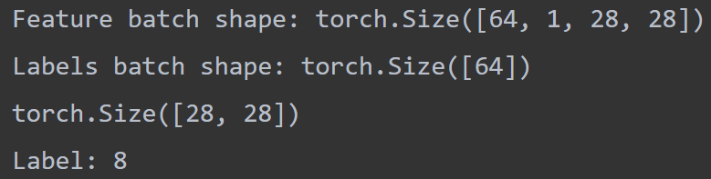
Sequence and Sampler Classes
For iterable datasets, the loading order of data is directly controlled by the user, allowing precise control over the samples returned in each batch, so there is no need to use the Sampler class.
For map-style datasets, since the indices can be non-integer, we can use the Sampler object to set the loading index sequence, i.e., to set an iterator over indices. If the shuffle parameter is set, the DataLoader will automatically create a sequential or random sampler. We can also pass a custom Sampler object through the sampler parameter.
Common Sampler objects include SequentialSampler and RandomSampler, which are created by passing the dataset to be sampled:
from torch.utils.data import DataLoader
from torch.utils.data import SequentialSampler, RandomSampler
from torchvision import datasets
from torchvision.transforms import ToTensor
training_data = datasets.FashionMNIST(    root="data",    train=True,    download=True,    transform=ToTensor())
test_data = datasets.FashionMNIST(    root="data",    train=False,    download=True,    transform=ToTensor())
train_sampler = RandomSampler(training_data)
test_sampler = SequentialSampler(test_data)
train_dataloader = DataLoader(training_data, batch_size=64, sampler=train_sampler)
test_dataloader = DataLoader(test_data, batch_size=64, sampler=test_sampler)
train_features, train_labels = next(iter(train_dataloader))
print(f"Feature batch shape: {train_features.size()}")
print(f"Labels batch shape: {train_labels.size()}")
test_features, test_labels = next(iter(test_dataloader))
print(f"Feature batch shape: {test_features.size()}")
print(f"Labels batch shape: {test_labels.size()}")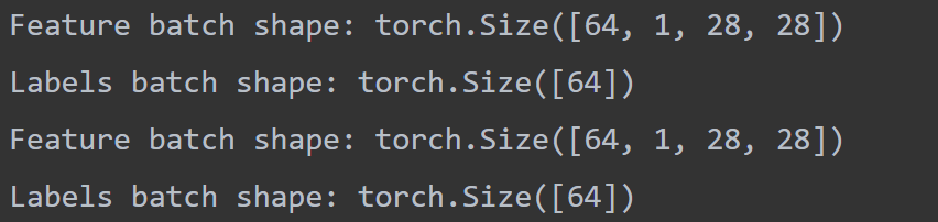
Batch Processing Function collate_fn
The batch processing function collate_fn is responsible for handling the samples in each sampled batch. The default collate_fn performs the following operations:
Adds a new dimension as the batch dimension;
Automatically converts NumPy arrays and Python numbers to PyTorch tensors;
Retains the original data structure; for example, if the input is a dictionary, it will output a dictionary containing the same keys but with values replaced by batched tensors (if they can be converted).
For instance, if the samples are tuples of 3-channel images and an integer category label, i.e., (image, class_index), the default collate_fn will convert such a list of tuples into a tuple containing batched image tensors and batched category label tensors.
We can also pass a manually written collate_fn function to customize the processing of the data, such as the padding operation mentioned earlier.
Due to the large amount of code in this article, for more content, please click the lower left corner of the article“Read the original text” to learn more!
Recruitment Requirements
Complete the production of robot-related videos that meet the requirements
Total duration must exceed 3 hours
The video content must be high-quality courses to ensure professionalism
Instructor Rewards
Enjoy revenue sharing from the course
Gift 2 courses from Guyue Academy’s premium courses (excluding training camps)
Contact Us
Add our staff WeChat: GYH-xiaogu