Essential Algorithms and Models in Mathematical Modeling

There are numerous models in mathematical modeling, but looking through the past competition problems of the National and American competitions, the main types frequently tested in mathematical modeling competitions are: evaluation type, prediction type, optimization type, and mechanism analysis type.

Evaluation type problems require assessing and analyzing a certain system, phenomenon, or plan. When modeling evaluation type problems, three aspects often need to be considered:

• What is the objective of the evaluation?

• What are the possible solutions to achieve the objective?

• What are the evaluation indicators/criteria?

Common models applied in evaluation modeling include: Analytic Hierarchy Process (AHP), Data Envelopment Analysis (DEA), Grey Relational Analysis, Fuzzy Comprehensive Evaluation, etc.

The difficulty in modeling prediction type problems lies in data collection and data cleaning. The quality of the data, feature selection, model selection, and tuning can greatly affect the accuracy of the prediction results.

Common models applied in prediction modeling include: Time Series Analysis, Grey Forecasting Model, Machine Learning Regression, etc.

Optimization type problems usually involve maximizing or minimizing an objective function, subject to some constraints, requiring the identification of feasible solutions that meet the constraints and finding an optimal solution among them. The optimal solution is the one that achieves the best value of the objective function under the given constraints.

Common models applied in optimization modeling include: Linear Programming, Dynamic Programming, Goal Programming, Integer Programming, etc.

Mechanism analysis type problems are based on the fundamental principles and theories of systems, such as physics, chemistry, and biology. They require a deep understanding of the internal mechanisms and interactions of the system and converting them into mathematical models. This requires a high level of expertise and is not recommended for beginners.

On May 31, 2023, SPSSPRO officially became the official sponsor and partner of the National College Students Mathematical Modeling Competition!

SPSSPRO will provide powerful data analysis software for the competition, welcome participants to use SPSSPRO in the competition!

Next, we will focus on explaining the commonly used models in evaluation, prediction, and optimization.

1. Evaluation Models

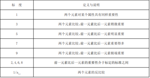
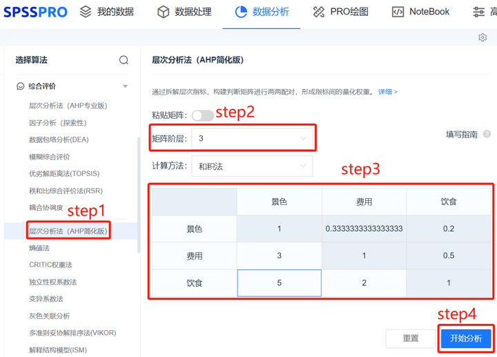
1.1 Analytic Hierarchy Process (AHP)

The Analytic Hierarchy Process is a decision analysis method that combines qualitative and quantitative approaches to solve complex multi-objective problems. This method integrates quantitative and qualitative analysis, using the decision-maker’s experience to judge the relative importance of the criteria that can achieve various measurement objectives.

When using the AHP method for decision-making, the following four steps need to be followed:

a. Establish a multi-level hierarchical structure model by creating a three-layer evaluation index system from top to bottom according to the dominance relationship: (1) The top layer, also known as the goal layer, is the primary criterion for the system’s evaluation. (2) The criteria layer includes the criteria and sub-criteria established to achieve the goal layer. (3) The bottom layer, also known as the alternative layer, includes the various plans and measures taken to achieve the goal.

b. Construct a pairwise comparison judgment matrix for elements at the same level, comparing them pairwise according to the elements of the upper level to establish the judgment matrix. Using pairwise comparison, let aij represent the degree of influence of element Bi compared to element Bj on goal A. To quantify the judgment, determine the relative importance of each element based on a scale of 1-9.

c. Weight Calculation

(1) Use the root method to calculate the approximate value of the eigenvector of the judgment matrix. (2) Normalize the eigenvector to obtain the weight vector.

d. Consistency Check

To ensure the correctness and rationality of the obtained weights, a consistency check is also needed.

The formula is: CR=CI/RI, where RI is the average random consistency index, CR is the consistency ratio, and CI is the measure of how much the judgment matrix deviates from consistency. When CR<0.1, the consistency of the judgment matrix can be considered acceptable.

e. Comprehensive Importance Calculation

The alternative with the highest weight is the optimal choice for achieving the goal.

Software Operation:

Step 1: Open the SPSSPRO free data analysis website, and select [Analytic Hierarchy Process (AHP Simplified Version)]

Step 2: Select the hierarchy of the judgment matrix (Note: the number of factors in the criteria layer equals the hierarchy of the judgment matrix. In this example, the criteria layer includes scenery, cost, and dining, so the hierarchy of the judgment matrix is 3.)

Step 3: Set the judgment matrix (the judgment matrix is a symmetric matrix), and set the elements of the judgment matrix.

Step 4: Click [Start Analysis], and the system will automatically analyze the results, which can be downloaded as a report.

1.2 Data Envelopment Analysis (DEA)

Data Envelopment Analysis is an effective method for evaluating multiple input and output indicators, comparing multiple inputs and outputs to obtain efficiency analysis, and can be widely used in performance evaluation.

Input: The input for Data Envelopment Analysis consists of input and output indicators (quantitative variables).

Output: Efficiency evaluation results, including specific input variables that need to be increased or decreased, and how to adjust output variables to achieve optimal efficiency.

The DEA model is divided into CCR model and BCC model, with the BCC model being the more commonly used one, and SPSSPRO defaults to the BCC model:

• The CCR model assumes that the DMU operates under constant returns to scale to measure overall efficiency.

• The BCC model assumes that the DMU operates under variable returns to scale to measure pure technical and scale efficiency.

Software Operation:

Step 1-3: Open the SPSSPRO free data analysis website and upload data.

Step 4: Select [Data Envelopment Analysis];

Step 5: Check the corresponding data format. [Data Envelopment Analysis] requires input indicators (quantitative variables >=1) to be placed first, followed by output indicators (quantitative variables >=1), and finally the index item (categorical variables <=1).

Step 6: Set the DEA type (Constant Returns to Scale (CCR) or Variable Returns to Scale (BCC)), in this example, choose the Variable Returns to Scale model (BCC).

Step 7: Click [Start Analysis], and the system will automatically analyze the results, which can be downloaded as a report.

1.3 Grey Relational Analysis

Grey Relational Analysis is a method for quantitatively describing and comparing the development trends of a system, based on determining the geometric similarity of reference data and several comparison data sequences to judge the closeness of their relationships, reflecting the degree of association between curves.

Its steps are as follows:

Step 1: Determine the characteristic sequence and the mother sequence.

Step 2: Dimensional normalization of the indicator data.

To accurately reflect the actual situation and eliminate influences caused by the differences in units and the discrepancies in the magnitude of values among different indicators, normalization of the indicators is necessary.

Step 3: Calculate the correlation coefficient.

Calculate the correlation coefficient for each comparison sequence corresponding to the reference sequence.

Step 4: Calculate the relational degree.

Calculate the weighted average of the correlation coefficients of each indicator with respect to the corresponding elements of the reference sequence, reflecting the relationship between each manipulated object and the reference sequence, referred to as the relational degree.

Step 5: Analyze the calculation results. Based on the size of the grey weighted relational degree, establish the relational order of each evaluation object. The larger the relational degree, the more important the evaluation object is to the evaluation standard.

Software Operation:

Step 1: Open the SPSSPRO free data analysis website and select [Grey Relational Analysis]

Step 5: Check the corresponding data format. [Grey Relational Analysis] requires the characteristic sequence to be a quantitative variable with at least one item; the mother sequence must be a quantitative variable with only one item.

Step 6: Set the dimensional processing method (including initial value normalization, mean normalization, no processing), and resolution coefficient (ρ is smaller, the resolution is greater, typically ρ is taken in the range of (0, 1), specific values can be determined based on the situation. When ρ ≤ 0.5463, the resolution is best, typically ρ = 0.5).

Step 7: Click [Start Analysis], and the system will automatically analyze the results, which can be downloaded as a report.

2. Prediction Modeling

2.1 Time Series Analysis

The full name of the ARIMA model is the Autoregressive Integrated Moving Average model, which is one of the most common statistical models used for time series forecasting.

The modeling process of the ARIMA model can be divided into the following four steps:

Step 1: Test the stationarity of the time series. Typically, the ADF or PP test methods are used to perform unit root tests on the original series. If the series does not meet the stationarity condition, it can be transformed through differencing or log differencing to convert a non-stationary time series into a stationary time series, and then construct the ARIMA model on the stationary time series;

Step 2: Determine the order of the model. By using some statistics that can describe the characteristics of the series, such as the autocorrelation (AC) coefficient and the partial autocorrelation (PAC) coefficient, preliminarily identify the possible forms of the model, and then select the best model from the available options based on criteria such as AIC;

Step 3: Parameter estimation and diagnostic testing. This includes testing the significance of the model parameters, the validity of the model itself, and testing whether the residual sequence is a white noise sequence. If the model passes the tests, the model specification is considered correct; otherwise, the model form must be re-specified and diagnostic testing must be repeated until the correct model form is obtained;

Step 4: Use the established ARIMA model for forecasting.

Software Operation:

Step 1: Open the SPSSPRO free data analysis website and select [Time Series Analysis (ARIMA)];

Step 2: Check the corresponding data format. [Time Series Analysis (ARIMA)] requires input of one time series data quantitative variable.

Step 3: Select the number of periods for backward forecasting.

Step 4: Click [Start Analysis], and the system will automatically analyze the results, which can be downloaded as a report.

2.2 Grey Forecasting Model

Grey forecasting is a method for predicting systems with uncertain factors. Grey forecasting identifies the degree of difference in development trends between system factors through correlation analysis and processes the original data to find patterns in system changes, generating a data sequence with strong regularity, and then establishes the corresponding differential equation model to predict the future development trends of the system.

The analysis steps are as follows:

Step 1: Before establishing the grey forecasting model, ensure the feasibility of the modeling method by performing a level comparison test on the known original data.

Step 2: Construct the data matrix B and data vector Y.

Step 3: Establish the model and solve for the generated and restored values. Based on the formula, the forecasting model can be obtained, and after cumulative reduction, the restored forecast values can be obtained.

Software Operation:

Step 1: Open the SPSSPRO free data analysis website and select [Grey Forecasting Model].

Step 2: Check the corresponding data format. [Grey Forecasting Model] requires input of one time series data quantitative variable.

Step 3: Select the number of periods for backward forecasting.

Step 4: Click [Start Analysis], and the system will automatically analyze the results, which can be downloaded as a report.

2.3 Machine Learning Regression Prediction

Machine learning regression prediction includes various models such as decision tree regression, random forest regression, BP neural network regression, etc. Here, we will take random forest regression as an example.

Random forest regression involves generating numerous decision trees through random sampling of the observation samples and feature variables in the modeling dataset. Each sampling result generates a tree, and each tree will produce rules and judgment values that conform to its attributes, while the forest integrates the rules and judgment values of all decision trees to achieve regression using the random forest algorithm.

The algorithm steps for random forest are as follows:

Step 1: Extract the training set from the original sample set. In each round, extract n training samples from the original sample set using the Bootstrapping method (sampling with replacement). A total of k rounds of extraction will yield k training sets (the k training sets are independent of each other).

Step 2: Use a training set to obtain a model in each round, resulting in k models from k training sets.

Step 3: For classification problems: use voting to obtain classification results from the k models obtained in the previous step; for regression problems, calculate the mean of the aforementioned models as the final result.

Software Operation:

Step 1: Open the SPSSPRO free data analysis website and select [Random Forest Regression].

Step 2: Check the corresponding data format and input the required data for [Random Forest Regression] (Note: it is recommended to encode categorical variables);

Step 3: Set parameters (the parameters in “More Settings” can be set in the client);

Step 4: Click [Start Analysis], and the system will automatically analyze the results, which can be downloaded as a report.

3. Optimization Models

3.1 Linear Programming

Linear programming problems have both the objective function and constraints as linear functions. The objective function can either be maximized or minimized, and the constraints can be represented by either less than or greater than inequalities.

3.2 Nonlinear Programming

If the objective function or constraints include nonlinear functions, such a programming problem is termed nonlinear programming. When only nonlinear objective functions and bounds on the values of unknowns are present, it is referred to as boundary constraint problems.

3.3 Integer Programming

Integer programming refers to linear programming problems where both the objective function and constraints are linear functions, and all variables are integers or Boolean types.

3.4 0-1 Programming

Programming where all variables are of Boolean type is referred to as 0-1 programming.

3.5 Heuristic Algorithms

Heuristic algorithms are constructed based on intuition or experience, providing a feasible solution to combinatorial optimization problems within acceptable costs (time and space). Common examples include: Genetic Algorithms, Particle Swarm Algorithms, Simulated Annealing Algorithms, Monte Carlo Algorithms.

Software Operation:

Step 1: Open the SPSSPRO free data analysis website and select the appropriate algorithm in the [Planning Solver] module.

Step 2: Construct the planning model.

Step 3: Solve the algorithm.

For more algorithm models and case data downloads, as well as case explanations, you can view and use them for free on SPSSPRO.