

Academic Dynamics
Dynamic Learning Graph Convolution Mechanism for
Short-Term Spatio-Temporal Traffic Flow Prediction Model

Short-term traffic flow prediction is a core branch of intelligent transportation systems and plays an important role in traffic management. Graph Convolutional Networks (GCN) are widely used in traffic prediction models, effectively handling the graphical structure data of road networks. However, in real life, the degree of influence between different road segments often varies, making manual analysis difficult. Traditional GCN methods rely on manually set adjacency matrices, which cannot dynamically adjust the weights of different road segments during the prediction process. To address this shortcoming, this article introduces a new Location Graph Convolutional Network (Location-GCN). Chen et al.[1] published this method in the journal Information Sciences in 2022, titled: “Spatial-temporal short-term traffic flow prediction model based on dynamical-learning graph convolution mechanism”. This method solves the problem by adding a new learnable matrix to the GCN, using the absolute values of this matrix to represent the differences in influence levels between different nodes.
Subsequently, the constructed traffic prediction model combines Long Short-Term Memory (LSTM) neural networks with Location-GCN to predict short-term traffic flow. Additionally, this method employs trigonometric function encoding to allow short-term input sequences to convey long-term periodic information. The following sections will provide a detailed introduction to this method.
1
Method Introduction
Traditional traffic flow prediction models, including GRU, LSTM, GCN, and GAT, focus on analyzing traffic patterns from a single perspective. However, changes in traffic flow in real life are influenced by spatial and temporal factors. To better analyze traffic data and achieve more accurate prediction performance, historical traffic data must be analyzed from both spatial and temporal perspectives. The method introduced in this paper constructs a short-term traffic flow prediction model by combining LSTM with GCN, and performs spatio-temporal analysis on historical data based on this model.
Location Graph Convolutional Network
(Location-GCN)
The Location Graph Convolutional Network (Location-GCN) can be described using the following equation:

A∈RN×N is the adjacency matrix, X∈RN×F represents the F feature input data of N nodes, Hl∈RN×F’(l≥1) represents the convolution result of F’ features, each row in the matrix Hl represents the traffic data of a single node in the road network, E is the identity matrix, and Wl is the trainable matrix.
Since the original trainable matrix Wl cannot be used for dynamic learning, this method proposes a trainable matrix Wmask to learn the different weights of two road nodes. By using Wmask, the improved GCN can automatically adjust the influence weights during the training process. Wmask is an N×N matrix, where N is the number of segment nodes. It has the same shape as the adjacency matrix A. The value at position [i,j] is the influence weight of i on j. Unlike traditional GCN mechanisms (which use A+E to obtain graph information between nodes in analysis), this matrix can independently change the influence weights of different segments through training, rather than just being set to 0 or 1.
To make the proposed GCN mechanism operational, the computation method of GCN must be altered. After the pattern learning of Wmask, the absolute value of each element in Wmask is used to create a new matrix Wabs, as the influence of upstream roads on downstream roads is usually positive. Then, it is multiplied by A+E, aiming to adjust the values of the adjacency matrix using weights trained from real data.
By using Wmask and Wabs, Location-GCN can analyze more detailed spatial patterns in traffic flow. A comparison between the traditional GCN and the proposed method is shown in Figure 1.
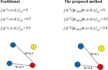
Figure 1 Comparison of Weight Calculation Results
In a road network with four nodes, nodes 2 and 3 are upstream nodes of node 0. Since traditional GCN can only represent the degree of influence between points as 0 or 1, the A+E weight values at positions [2,0] and [3,0] are both 0.5 after normalization D-1, leading to the assumption that nodes 2 and 3 have equal influence weight on node 0. However, the improved method allows the model to learn the differences in influence during training, enabling the convolution operation to obtain this knowledge through multiplication with Wabs.
The Proposed Model
Loc-GCLSTM
To better handle periodic patterns in historical traffic data, Loc-GCLSTM first applies trigonometric function encoding to the data, using the periodic characteristics of sine and cosine functions to describe periodic information in traffic patterns. Subsequently, the data is input into the Location GCN layer, utilizing the trainable matrix to learn the different influence levels of various upstream segments on each downstream segment. Finally, the spatial analysis of location-GCN is combined with the temporal analysis of LSTM for prediction. The structure of the proposed model is shown in Figure 2.
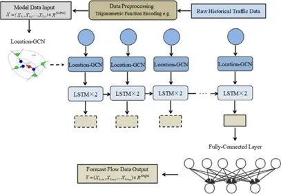
Figure 2 Structure of the Loc-GCLSTM Model
2
Result Evaluation
Two different datasets, domestic and international (OpenITS and METR-LA), were selected for model training. The input features from the OpenITS dataset include traffic flow, average speed, flow density, proportions of large and regular vehicles, timestamps (5-minute intervals, 1-day cycle), hours (1-hour intervals, 1-week cycle), number of lanes, and weather. In the METR-LA dataset, traffic flow, timestamps (5-minute intervals, 1-day cycle), and hours (1-hour intervals, 1-week cycle) were selected. The timestamp and hour data were encoded using trigonometric functions, and the weather was numerically encoded. After Z-score normalization, this data was used as input for model training.
01
Prediction Results
Table 1 shows the accuracy comparison of five evaluation metrics in the model trained using the OpenITS dataset. According to all metrics, Loc-GCLSTM achieved the best results. Due to the lack of long-term dependency analysis in LSTM, the performance of the STGCN spatio-temporal model is inferior to that of LSTM.
Table 2 shows the accuracy comparison of five evaluation metrics in the model trained using the METR-LA dataset. Overall, according to all standards, Loc-GCLSTM outperformed other methods. Since it predicts traffic flow for the next 12 five-minute intervals, the LSTM model also performed well on this dataset, fully demonstrating the excellence of LSTM in executing multiple sequence prediction tasks.
Table 1 Prediction Results of the OpenITS Dataset
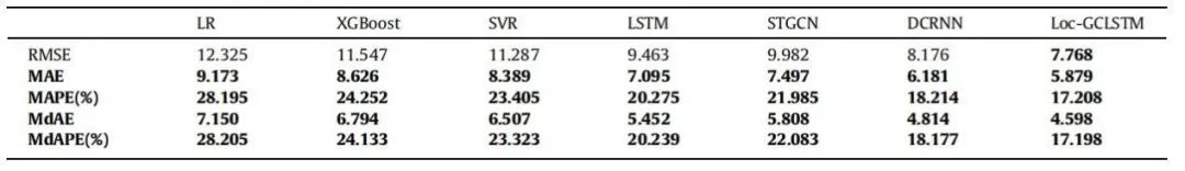
Table 2 Prediction Results of the METR-LA Dataset
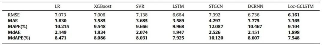
Figure 3 shows the prediction error distribution of LSTM, DCRNN, and Loc-GCLSTM on the OpenITS and METR-LA datasets, where the x-axis represents the error between predicted results and actual data, and the y-axis represents the error distribution. Clearly, the distribution of Loc-GCLSTM is denser around 0, indicating that in most cases, Loc-GCLSTM results are more accurate. The x-axis is also denser, indicating that Loc-GCLSTM is more stable in prediction accuracy.
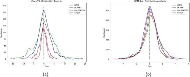
Figure 3 Error Distribution Chart
02
Convergence Speed
After training, the prediction results of each model were recorded. RMSE was used to evaluate convergence speed. Figure 4 shows the evaluation results, where Loc-GCLSTM achieved the fastest convergence speed and the most stable, highest prediction accuracy on the OpenITS and METR-LA datasets.
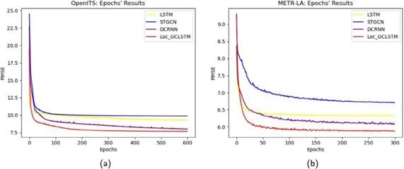
Figure 4 Convergence Speed of Different Methods
03
Segmented Prediction Results
In the evaluation of the OpenITS dataset, the first and fourth observation nodes selected data from July 5, July 7, and July 16, during the time periods of 7:30-9:30 and 11:30-13:30, comparing the prediction results of LSTM and Loc-GCLSTM with actual data. In Figure 5, the green line represents actual data, the blue line represents the prediction results of LSTM, and the red line represents the prediction results of Loc-GCLSTM. The results indicate that the Loc-GCLSTM predictions are closer to the actual data.
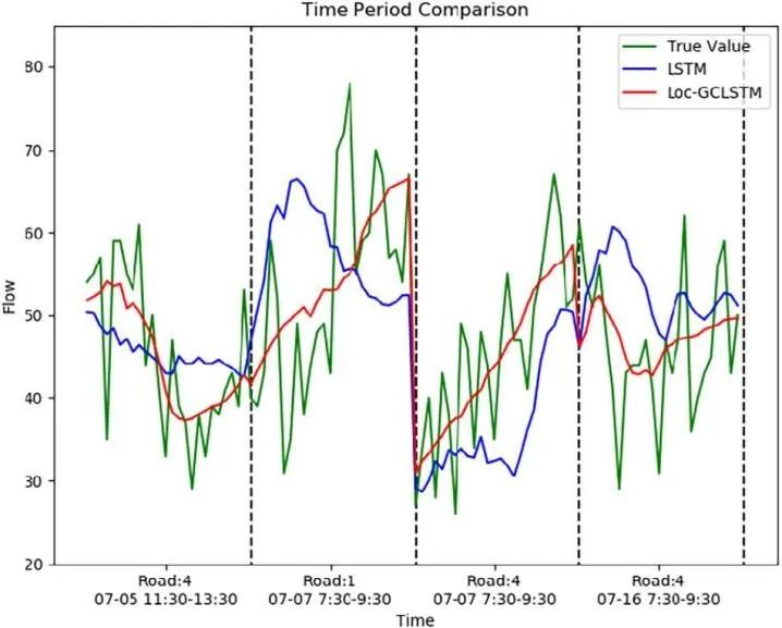
Figure 5 Comparison of Segmented Prediction Results of Different Models
04
Prediction Accuracy for Each Road
As shown in Figure 6, in the evaluation of the OpenITS dataset, using RMSE, MAPE, and MAE metrics, the prediction accuracy of Loc-GCLSTM on each road was compared with LSTM, DCRNN, and STGCN. The results indicate that Loc-GCLSTM outperforms other methods and is suitable for the majority of real road traffic predictions.
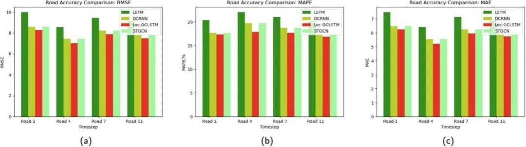
Figure 6 Comparison of Prediction Results for Different Roads Using Different Methods
3
Conclusion
This article provides a detailed introduction to a novel short-term traffic flow prediction model named Loc-GCLSTM. This model combines Loc-GCN with LSTM for predictions from both temporal and spatial perspectives. However, while Loc-GCN can only consider the differences in influence between different road segments, it cannot evaluate how the influence weights between different nodes change over time. Nevertheless, all results indicate that this method is superior to others in short-term traffic flow prediction and can provide references for subsequent research.
References
[1] Chen Zhijun, Lu Zhe, Chen Qiushi, et al (2022). Spatial-temporal short-term traffic flow prediction model based on dynamical-learning graph convolution mechanism. Information Sciences, 611, 522-539.
Contributed by: Li Yuankai