Comprehensive Summary of Machine Learning Models

About 10,000 words, recommended reading time 20 minutes.
This article introduces the models of machine learning.

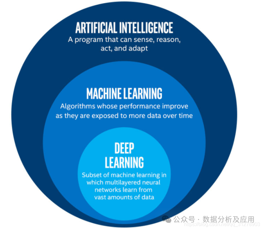
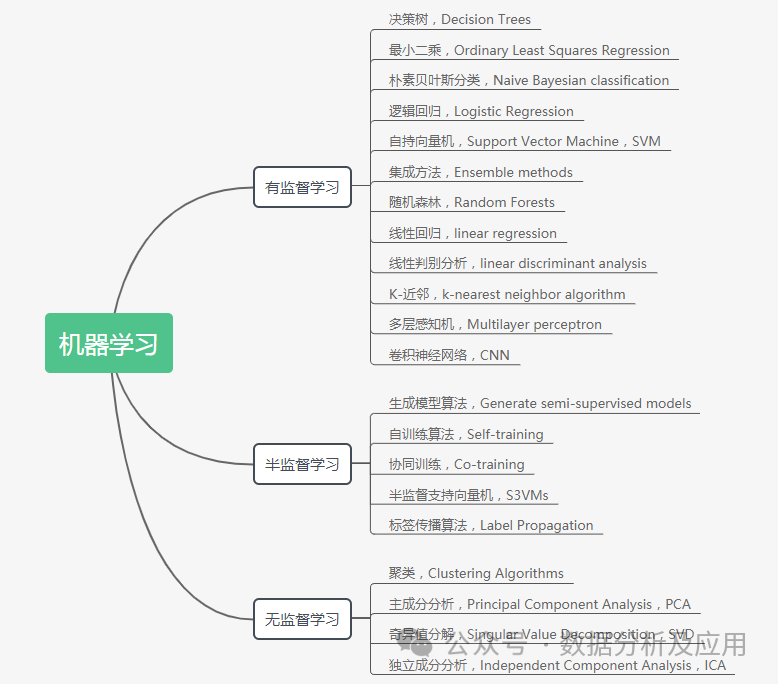
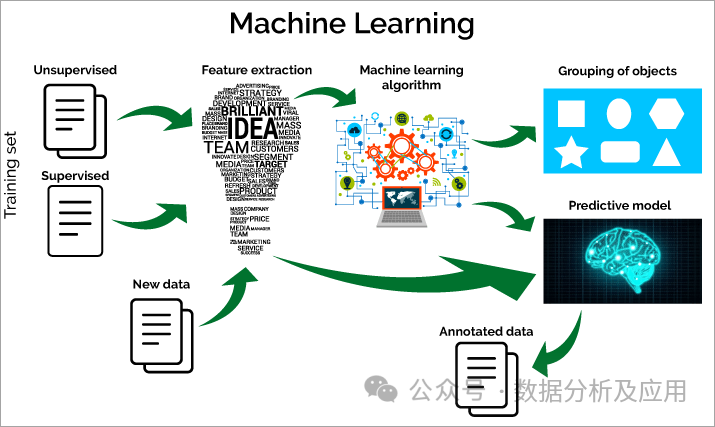
Machine learning is the process of allowing computers to automatically extract rules and patterns from data, thereby completing specific tasks. According to model types, machine learning is mainly divided into three categories: supervised learning models, semi-supervised learning, and unsupervised learning models. (In addition to the aforementioned three categories, there is reinforcement learning, which allows computers to automatically interact with the environment to learn strategies to maximize rewards.)

Different machine learning models have their specific principles and are suitable for different tasks and scenarios. Below, we systematically review the machine learning models and their algorithmic principles!

1. Supervised Learning

Supervised learning is an important method in machine learning, which utilizes labeled training data with expert annotations to learn the function mapping from input variable X to output variable Y. In this process, each input sample is associated with a corresponding output label. Through these associated samples and labels, machines can learn the mapping relationship between input and output.

Specifically, supervised learning can be divided into two types of problems:

1. Classification Problems: These problems mainly predict the category to which a sample belongs. Categories are usually discrete, such as determining gender or predicting stock price fluctuations. In classification problems, machine learning models classify new input samples into corresponding categories by learning the relationship between classification labels and input features.
2. Regression Problems: These problems mainly predict the real number output of a sample. Output values are usually continuous, such as predicting housing prices or stock prices. In regression problems, machine learning models predict continuous values for new input samples by learning the relationship between input features and output values.

Linear Regression

Model Principle:

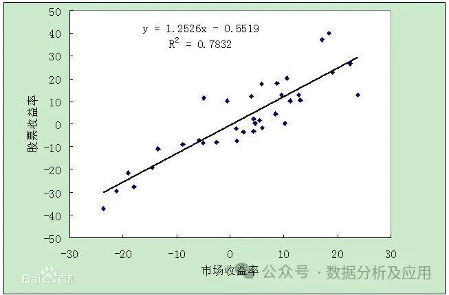
Linear regression is a simple and effective regression analysis method. Its basic principle is to fit a line by minimizing the sum of squared errors between predicted and actual values, thereby predicting future values. The linear regression model can be represented by a formula: y = wx + b, where w is the slope and b is the intercept. The linear regression model assumes a linear relationship between the data and finds the best-fit line by minimizing the sum of squared errors.

Model Training:

The training process of the linear regression model is the process of minimizing the sum of squared errors, typically using optimization algorithms such as gradient descent to find the best w and b. During training, we need to calculate the vertical distance from each sample point to the fitted line and update w and b to reduce the error. After training is complete, we can use this model to predict new data points.

Advantages:

1. Simple and Understandable: The linear regression model is easy to understand and implement.
2. High Computational Efficiency: The linear regression model has a low computational complexity and can quickly process large datasets.
3. Strong Interpretability: The linear regression model can explain the impact of variables on results through coefficients.

Disadvantages:

1. Assumption Limitations: The linear regression model assumes a linear relationship between data, which may not apply to all cases.
2. Sensitive to Outliers: The linear regression model is sensitive to outliers, which can easily affect the model.
3. Cannot Handle Non-linear Problems: The linear regression model cannot handle non-linear problems and performs poorly on non-linear data.

Usage Scenarios:

The linear regression model is suitable for low-dimensional cases where there is no multicollinearity among dimensions, making it suitable for linearly separable datasets. For example, it can be used to predict housing prices, stock prices, and other continuous numerical data.

Example Code:

# Import required libraries

import numpy as np

from sklearn.model_selection import train_test_split

from sklearn.linear_model import LinearRegression

from sklearn.metrics import mean_squared_error

# Generate simulated data. Then use the model to learn to fit and predict these data

np.random.seed(0)

X = np.random.rand(100, 1) * 10

y = 3 * X + 2 + np.random.randn(100) * 0.1

# Split the dataset into training and testing sets

X_train, X_test, y_train, y_test = train_test_split(X, y, test_size=0.2, random_state=42)

# Create linear regression model object

model = LinearRegression()

# Train the model using training data

model.fit(X_train, y_train)

# Predict on the test set

y_pred = model.predict(X_test)

# Calculate mean squared error (MSE) as a performance evaluation metric for the model

mse = mean_squared_error(y_test, y_pred)

print(‘Mean Squared Error (MSE):’, mse)

Logistic Regression

Model Principle:

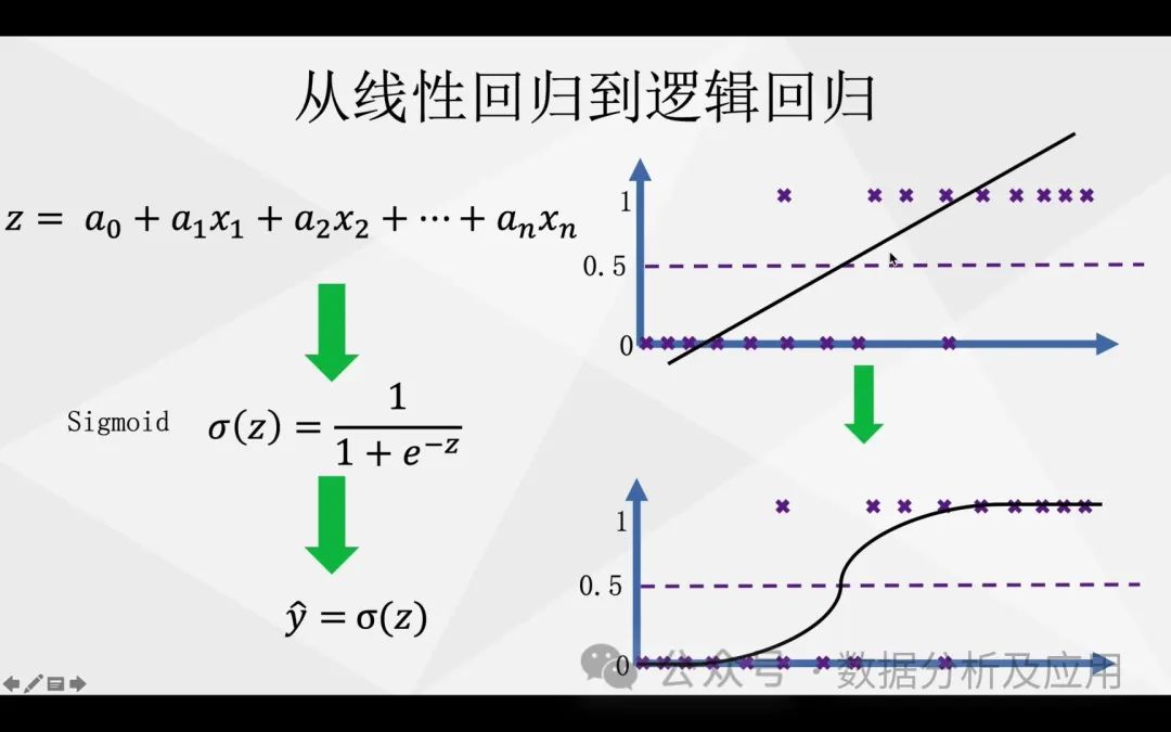
Logistic regression is a regression analysis method used to solve classification problems. It describes the relationship between input variables and output variables by adding a logistic function (sigmoid) based on linear regression. The logistic regression model is typically represented as y = sigmoid(wx + b), where sigmoid is a function that maps any value to between 0 and 1, w is the slope, and b is the intercept. The logistic regression model assumes a probability distribution exists between data and can find the best-fitting parameters by maximizing the likelihood function.

Model Training:

The training process of the logistic regression model is the process of maximizing the likelihood function, typically using optimization algorithms such as gradient descent to find the best w and b. During training, we need to calculate the vertical distance from each sample point to the fitted curve and update w and b to increase the probability of correct classification while reducing the probability of incorrect classification. After training is complete, we can use this model to predict the classification results of new data points.

Advantages:

1. Suitable for Classification Problems: The logistic regression model is suitable for solving classification problems, especially binary classification problems.
2. Simple and Understandable: The logistic regression model is relatively simple and easy to understand and implement.
3. High Computational Efficiency: The logistic regression model has low computational complexity and can quickly process large datasets.

Disadvantages:

1. Assumption Limitations: The logistic regression model assumes a linear relationship between data, which may not apply to all cases.
2. Sensitive to Outliers: The logistic regression model is sensitive to outliers, which can easily affect the model.
3. Cannot Handle Non-linear Problems: The logistic regression model cannot handle non-linear problems and performs poorly on non-linear data.

Usage Scenarios:

The logistic regression model is suitable for solving binary classification problems, such as spam filtering and fraud detection.

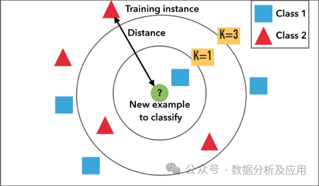
KNN (K-Nearest Neighbors)

Model Principle:

KNN is an instance-based learning algorithm. Its basic idea is that if a sample point belongs to the majority class of its k nearest neighbors in feature space, then that sample point also belongs to that class. The KNN algorithm classifies or regresses by measuring the distances between different data points.

Model Training:

The training process of the KNN algorithm does not require an explicit training phase, as its training data is simply the data stored in memory. During the classification phase, for a new input sample, the algorithm calculates the distance to each sample in the training set and selects the k nearest samples. Finally, it decides the class of the new sample based on the majority class of these k nearest samples. In the regression phase, the algorithm simply takes the average of the k nearest samples as the predicted value.

Advantages:

1. Simple and Understandable: The KNN algorithm is simple and easy to understand and implement.
2. Robust to Outliers: Since KNN is instance-based learning rather than parameter learning, it is relatively robust to outliers and noise.
3. Can Handle Non-linear Problems: KNN performs well on non-linear problems by measuring distances between different data points for classification or regression.

Disadvantages:

1. High Computational Load: The KNN algorithm has high computational complexity, especially on large datasets, resulting in significant computation.
2. Choosing an Appropriate K Value: The choice of K value significantly affects the performance of the KNN algorithm; if chosen improperly, it may lead to poor classification results.
3. Sensitive to High-dimensional Data: In high-dimensional space, all data points may be considered close together, leading to a decline in KNN’s performance.

Usage Scenarios:

The KNN algorithm is suitable for various classification and regression problems, especially in cases where the sample space is close to a low-dimensional subspace. It has extensive applications in text classification, image recognition, recommendation systems, etc.

Decision Tree

Model Principle:

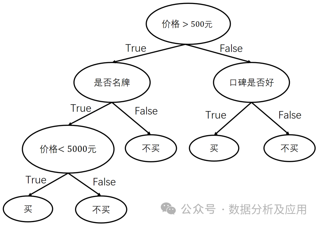
A decision tree is a tree-structured classification and regression algorithm. It consists of multiple nodes, where each node represents a judgment on a feature attribute, each branch represents a possible attribute value, and each leaf node represents a class or decision result. Decision trees learn the classification or regression rules of data by recursively constructing decision trees.

Model Training:

The training process of a decision tree starts from the root node and partitions the dataset by comparing feature attributes. For each node, the algorithm selects the optimal feature for partitioning, maximizing the purity of the partitioned dataset. After partitioning, the algorithm recursively performs the same operation on each child node until stopping criteria are met. After training is complete, we can use this decision tree to predict the classification or regression results of new data points.

Advantages:

1. Strong Interpretability: The decision tree model can generate easily understandable rules, making its results more acceptable to users.

Disadvantages:

1. Sensitive to Feature Selection: The decision tree algorithm is highly sensitive to feature selection; different feature selections may lead to entirely different decision trees, which may degrade the model’s generalization performance.
2. Prone to Overfitting: If there is noise or outliers in the training data, decision trees may overfit these data, leading to poor performance on new datasets.
3. Poor Handling of Continuous Features: The decision tree algorithm is not flexible in handling continuous features, which may lead to unnecessary branches or overfitting.

Usage Scenarios:

The decision tree algorithm is suitable for classification and regression problems, especially for feature selection and feature engineering. It has extensive applications in finance, healthcare, and industry, such as credit scoring, disease diagnosis, and fault detection.

Naive Bayes

Model Principle:

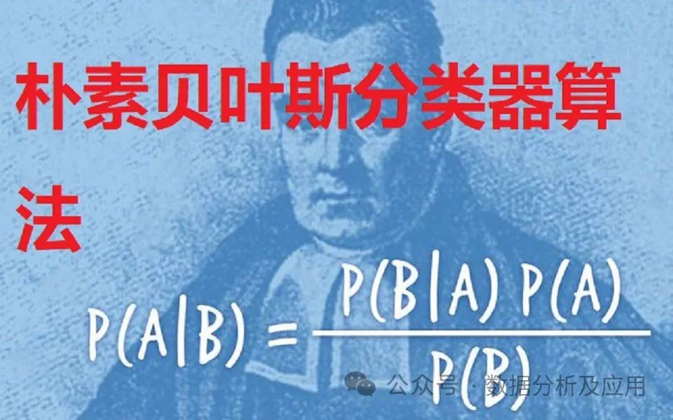
Naive Bayes is a classification method based on Bayes’ theorem and the assumption of independence between features. Its basic idea is to calculate the probabilities of each category for a given input sample and choose the category with the highest probability as the prediction result. Naive Bayes assumes that each feature is independent given the category. It calculates the probabilities of given data using Bayes’ theorem and determines classification based on maximum probability.

Model Training:

The training process of the Naive Bayes model involves calculating the prior probabilities of each category and the conditional probabilities of each feature given each category. During training, we count each category and each feature and use these counts to calculate probabilities. In the prediction phase, the algorithm calculates the posterior probabilities for each category based on the probabilities calculated during training and selects the category with the highest probability as the prediction result.

Advantages:

1. Simple and Understandable: The Naive Bayes model is simple and easy to understand and implement.
2. High Accuracy: On certain datasets, the Naive Bayes algorithm has a high classification accuracy.
3. Robust to Missing and Outlier Values: Since Naive Bayes is a probability-based classification method, it is less sensitive to missing and outlier values.

Disadvantages:

1. Assumption Limitations: The Naive Bayes algorithm assumes independence between features, which may not apply to all cases.
2. Poor Performance on High-dimensional Data: For high-dimensional data, the performance of the Naive Bayes algorithm may decline, as each feature requires probability calculations.
3. Sensitive to Data Scale: The Naive Bayes algorithm is sensitive to data scale; if the training data is small, it may lead to overfitting.

Usage Scenarios:

The Naive Bayes algorithm is suitable for applications such as text classification and spam filtering. Its assumption of independence between features makes it effective in handling text data.

Neural Networks (DNN)

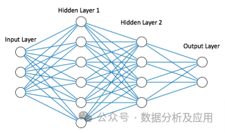
Neural Network Model Principle:

A neural network is a machine learning model that simulates the transmission process between neurons in the human brain. It consists of multiple neurons, where each neuron receives input signals and calculates output values. The connections between multiple neurons have parameters such as weights and thresholds. Neural networks learn effective representations of input data through training and use these representations for classification, prediction, or other tasks.

Model Training:

The training process of a neural network involves adjusting parameters such as weights and thresholds so that the neural network’s output is as close as possible to the true values. During training, methods such as backpropagation are typically used to calculate the error for each neuron and update the weights and thresholds based on the error. After training is complete, we can use this neural network to predict the classification or regression results of new data points.

Advantages:

1. Powerful Non-linear Mapping Ability: Neural networks can learn and express complex non-linear relationships, which is difficult for other models.
2. Strong Fault Tolerance: Due to the redundancy of neurons and connections, neural networks have strong fault tolerance to outliers and noise.
3. Can Handle Large-scale Data: Neural networks can process large-scale datasets, and their performance often surpasses that of other models when the dataset is large.

Disadvantages:

1. Long Training Time: The training time for neural networks is typically long, especially on large datasets, which may require substantial computational resources and expertise.
2. Prone to Local Optima: Due to the large parameter space of neural networks, it is easy to fall into local optima during training, leading to poor model performance.
3. Sensitive to Parameter Tuning: The performance of neural networks is very sensitive to parameters (such as learning rate, batch size, etc.), and inappropriate parameters may lead to poor model performance.

Usage Scenarios:

Neural networks are suitable for various complex data and problems, especially in fields such as image recognition, speech recognition, natural language processing, and game AI. They are also suitable for solving problems that other models cannot handle or perform poorly on.

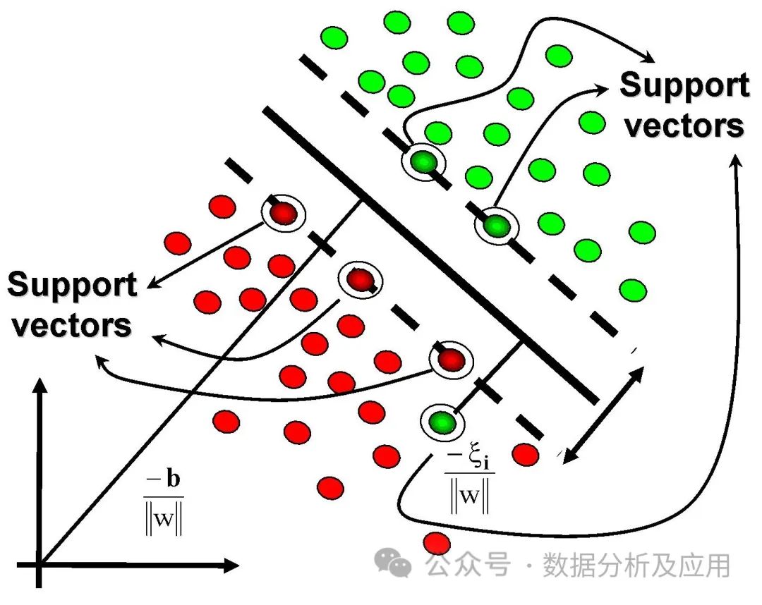
Support Vector Machines (SVM)

Model Principle:

Support Vector Machines are a classification and regression machine learning model that achieves classification or regression by finding decision boundaries that maximize the separation of data points from different categories. SVM uses kernel functions to map input space into high-dimensional feature space and constructs decision boundaries in that space.

Model Training:

The training process of SVM is about finding the optimal decision boundary. During training, the algorithm finds the hyperplane that maximally separates the data points while considering constraints and error terms. After training is complete, we can use this SVM model to predict the classification or regression results of new data points.

Advantages:

1. Good Classification Performance: SVM typically performs well in classification, especially when handling linearly separable datasets.
2. Robust to Outliers and Noise: SVM is robust to outliers and noise, as they mainly affect the error term during training.
3. Strong Interpretability: The decision boundary of SVM is easy to interpret and can provide useful information about the data.

Disadvantages:

1. Sensitive to Parameters and Kernel Functions: The performance of SVM is very sensitive to parameters (such as penalty coefficients, kernel functions, etc.) and the choice of kernel functions.
2. Low Efficiency on Large Datasets: For large datasets, the training time of SVM may be long and require significant storage space.
3. Not Suitable for Non-linear Problems: For non-linear problems, SVM requires using kernel functions to map input space to high-dimensional feature space, which may reduce computational efficiency.

Usage Scenarios:

SVM is suitable for various classification and regression problems, especially for handling linearly separable datasets. It has extensive applications in text classification, bioinformatics, finance, and more. Additionally, SVM can be used for specific problems such as anomaly detection and multi-class classification.

Ensemble Learning Models

Model Principle:

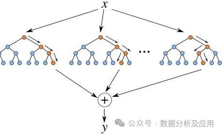
Ensemble learning does not refer to a single model but to a machine learning technique that improves prediction accuracy and stability by combining multiple base learners (such as decision trees, neural networks, etc.). The basic idea of ensemble learning is to use the predictions of multiple base learners for voting or weighted averaging to obtain better prediction results. Common models include GBDT, Random Forest, XGBOOST, etc.:

GBDT (Gradient Boosting Decision Tree) is a boosting algorithm based on CART regression trees. It uses an additive model and trains a set of CART regression trees serially to build a strong learner. Each new tree fits the negative gradient direction of the current loss function and sums the predictions of all regression trees to obtain the final regression result. For classification problems, sigmoid or softmax functions can be applied to obtain binary or multi-class results.

AdaBoost adjusts the weights of learners so that those with a lower error rate receive a higher weight, thus generating a strong learner. In both regression and classification problems, the calculation of error rates differs. Classification problems typically use a 0/1 loss function, while regression problems use squared loss or linear loss functions.

XGBoost is an efficient implementation of GBDT that adds a regularization term to the loss function. Additionally, since some loss functions are difficult to derive, XGBoost uses the second-order Taylor expansion of the loss function for fitting.

LightGBM is another efficient implementation of XGBoost. Its main idea is to discretize continuous floating-point features and construct histograms. By traversing training data, it calculates the cumulative statistics of each discrete value in the histogram for feature selection. During feature selection, it only needs to traverse the optimal split points based on the histogram’s discrete values. Additionally, LightGBM uses a depth-limited leaf-wise growth strategy to save time and space costs.

Model Training:

The training process of ensemble learning involves generating multiple base learners and combining them. During training, methods such as bagging and boosting are typically used to generate different base learners and adjust their weights and parameters. After training is complete, we can use this ensemble model to predict the classification or regression results of new data points.

Advantages:

1. High Predictive Accuracy: Ensemble learning can often achieve higher predictive accuracy by combining the advantages of multiple base learners.
2. Good Stability: Ensemble learning can reduce the risk of overfitting or underfitting of a single model, improving the model’s stability.
3. Suitable for Handling Large Datasets: Ensemble learning can effectively handle large-scale datasets by dividing the dataset into multiple subsets for training different base learners.

Disadvantages:

1. High Computational Complexity: Ensemble learning requires training multiple base learners, resulting in higher computational complexity and requiring more computational resources and time.
2. Difficulty in Parameter Tuning: The performance of ensemble learning is very sensitive to parameters (such as the number of base learners, weights, etc.) and selection methods, making tuning challenging.
3. Potential Over-complexity: Ensemble learning may lead to overly complex models, increasing the risk of overfitting.

Usage Scenarios:

Ensemble learning is suitable for various classification and regression problems, especially for handling large-scale datasets and addressing overfitting issues. It has extensive applications in finance, healthcare, and industry, such as credit scoring, disease diagnosis, and fault detection. Ensemble learning models typically have strong fitting effects, like XGBOOST, which is often the winning tool in data mining competitions.

2. Unsupervised Learning

Unsupervised learning is a machine learning method that uses unlabeled data for training, allowing the model to extract useful information or structures from the data autonomously. Unlike supervised learning, unsupervised learning does not have explicit labels to guide the model’s predictions. Common unsupervised learning algorithms include clustering, PCA dimensionality reduction, and isolation forest anomaly detection.

Unsupervised learning has extensive applications in many fields, such as market segmentation, recommendation systems, and anomaly detection. By using unsupervised learning, we can extract useful information from large amounts of unlabeled data, thus better understanding the data and making corresponding decisions.

K-means Clustering

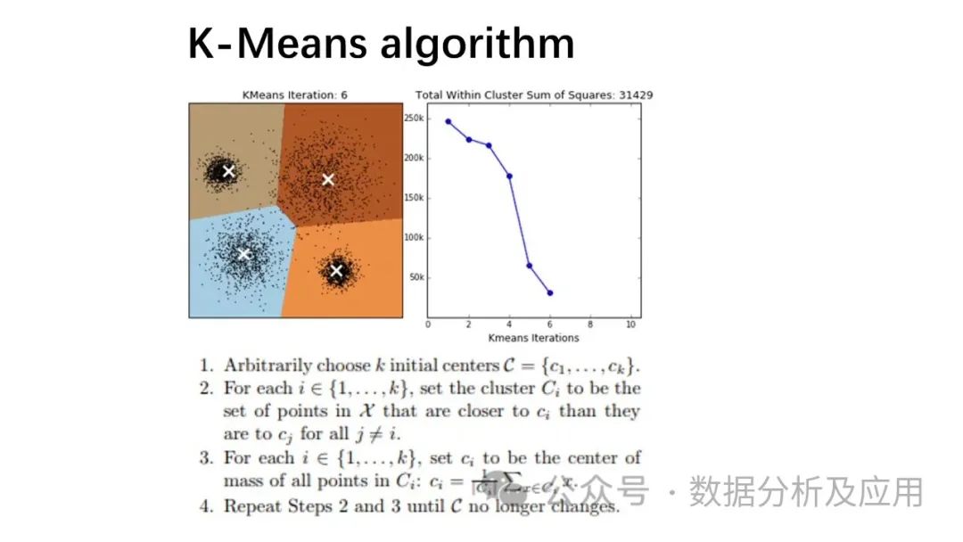
K-means clustering is an unsupervised learning algorithm. Its basic principle is to iteratively partition the dataset into K clusters, minimizing the sum of distances between each data point and the center of its cluster.

Model Training:

The training process of K-means can be divided into the following steps:

1. Select Initial Cluster Centers: Randomly select K data points as initial cluster centers.
2. Assign Data Points to Nearest Cluster Centers: Based on the distance between each data point and the cluster centers, assign data points to the nearest corresponding clusters.
3. Update Cluster Centers: Recalculate the center of each cluster, setting it as the average of all data points in that cluster.
4. Repeat Steps 2 and 3 until the cluster centers no longer change significantly or reach a preset number of iterations.

Advantages:

1. Simple and Understandable: The K-means algorithm is simple and easy to understand and implement.
2. Strong Interpretability: The clustering results of K-means have a certain interpretability, as each cluster can be represented by its center.
3. Robust to Outliers: The K-means algorithm is not highly sensitive to outliers, as outliers only affect individual clusters and have a smaller impact on the overall clustering results.
4. Suitable for Large Datasets: The K-means algorithm is suitable for handling large-scale datasets, as it only requires calculating distances between data points and cluster centers without considering complex relationships between data points.

Disadvantages:

1. Sensitive to Initial Cluster Centers: The K-means algorithm is sensitive to the choice of initial cluster centers; different initial centers may lead to different clustering results.
2. Prone to Local Optima: The K-means algorithm may fall into local optima rather than global optima.
3. Requires Predefined Number of Clusters K: The K-means algorithm requires the number of clusters K to be predefined, which can sometimes be difficult to determine.
4. Sensitive to Non-spherical Clusters and Empty Clusters: The K-means algorithm is sensitive to non-spherical clusters and empty clusters, which may lead to inaccurate clustering results.

Usage Scenarios:

K-means is suitable for various scenarios requiring clustering, such as market segmentation, image segmentation, and social network analysis. It can partition datasets into several clusters with similar features, facilitating further analysis and mining. Additionally, K-means can be used for anomaly detection and preprocessing in classification tasks.

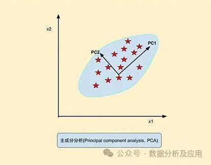
PCA (Principal Component Analysis)

PCA (Principal Component Analysis) is a commonly used dimensionality reduction method. Its basic principle is to linearly transform the original features, projecting the data onto an orthogonal coordinate system formed by the variance of the original features, retaining the direction of maximum variance to eliminate irrelevant or redundant features and achieve dimensionality reduction.

Model Training:

The training process of PCA includes the following steps:

1. Standardization: Standardize the original features so that they have a mean of 0 and a variance of 1.
2. Calculate Covariance Matrix: Calculate the covariance matrix of the standardized dataset.
3. Calculate Eigenvalues and Eigenvectors: Perform eigenvalue decomposition on the covariance matrix to obtain eigenvalues and eigenvectors.
4. Select Principal Components: Select the top k eigenvectors corresponding to the largest eigenvalues based on the number of principal components set, forming a new coordinate system.
5. Project Data: Project the original data onto the new coordinate system to obtain the reduced dimensional data.

Advantages:

1. No Parameter Limits: PCA is an unsupervised learning method that does not require manual parameter setting or intervention based on empirical models; the final result is only related to the data.
2. Good Dimensionality Reduction Effect: PCA effectively reduces data dimensions by retaining the direction of maximum variance and removing irrelevant or redundant features.
3. Retains Main Information: PCA transforms the weights and coordinate system of the original features so that the reduced data still reflects the main information of the original data.
4. Good Visualization Effect: PCA can map high-dimensional data to low-dimensional space, facilitating visual display of data for human observation and understanding.

Disadvantages:

1. Sensitive to Data Distribution: PCA assumes that data conforms to a Gaussian distribution; if the data distribution significantly deviates from Gaussian, it may lead to poor dimensionality reduction effects.
2. Cannot Handle Non-linear Problems: PCA is a linear dimensionality reduction method and may not yield good dimensionality reduction effects for non-linear problems.
3. Sensitive to Outliers: PCA is sensitive to outliers, which may affect the calculation of the covariance matrix and the results of eigenvalue decomposition.

Usage Scenarios:

PCA is suitable for various scenarios requiring dimensionality reduction, such as image processing, text analysis, natural language processing, and machine learning. It can reduce high-dimensional data to low-dimensional space, facilitating visualization, classification, clustering, and other tasks. Additionally, PCA can be used for data preprocessing and feature selection, removing irrelevant or redundant features to enhance the model’s generalization ability and computational efficiency.

Example Code:

The following is an example code for K-means clustering using the iris dataset:

from sklearn.cluster import KMeans

from sklearn.datasets import load_iris

import matplotlib.pyplot as plt

### First load the iris dataset and store it in variables X and y. Then create a KMeans object and specify the number of clusters as 3. Next, train the model with the training data and obtain the cluster centers and the cluster labels for each sample. Finally, use the matplotlib library to visualize the clustering results, where different colored points represent samples from different clusters, and the red points represent the cluster center.

# Load the iris dataset

iris = load_iris()

X = iris.data

y = iris.target

# Create KMeans object, specify number of clusters as 3

kmeans = KMeans(n_clusters=3)

# Train the model using training data

kmeans.fit(X)

# Get cluster centers

centers = kmeans.cluster_centers_

# Get the cluster labels for each sample

labels = kmeans.labels_

# Visualize clustering results

plt.scatter(X[:, 0], X[:, 1], c=labels, s=50, cmap=’viridis’)

plt.scatter(centers[:, 0], centers[:, 1], c=’red’, s=200, alpha=0.5) # Draw cluster center

plt.show()

Isolation Forest

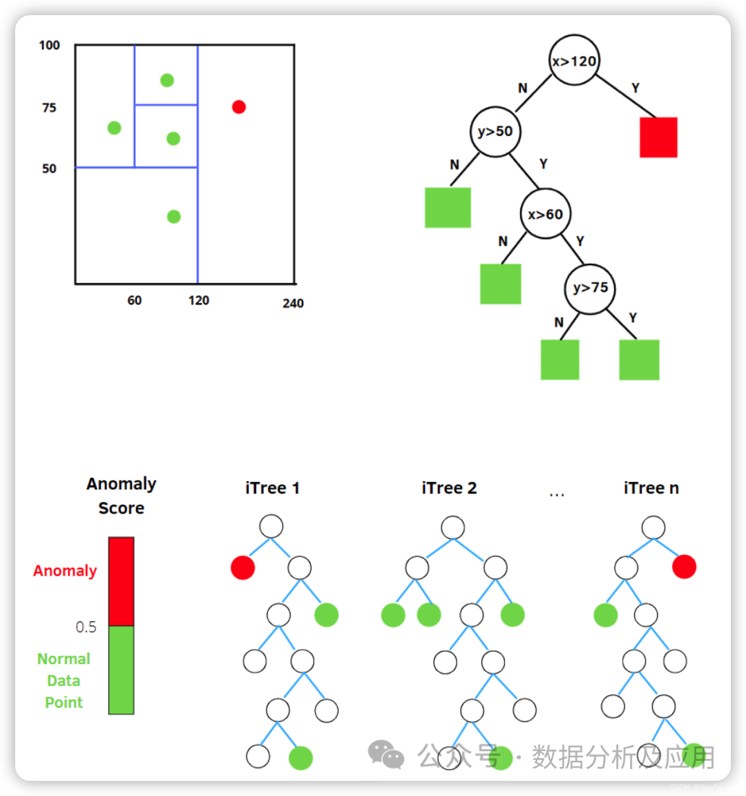
Isolation Forest is a classic anomaly detection algorithm. Its basic principle is to use binary trees to construct an anomaly detection model. During training, the isolation forest constructs binary trees by randomly selecting features and samples, splitting the data at each node based on features and thresholds into left and right subsets. By using multiple independently constructed binary trees, the isolation forest can calculate the average path length for each data point and determine whether it is an anomaly based on that length.

Model Training:

The training process of the isolation forest includes the following steps:

1. Sampling: Randomly sample a certain number of samples from the training dataset without replacement to serve as training data.
2. Construct Binary Trees: For each isolation tree, randomly select a feature and threshold to split the data into left and right subsets. Repeat this process until a preset stopping condition is met (such as tree height limit or the number of samples in the subset being less than a certain threshold).
3. Ensemble Multiple Isolation Trees: Repeat the above steps multiple times to construct multiple independent isolation trees.
4. Calculate Average Path Length: For each data point, calculate its average path length in all isolation trees.
5. Determine Anomalous Points: Based on a set threshold, data points with shorter average path lengths are determined to be anomalous.

Advantages:

1. Strong Stability: Due to the random selection of samples during the construction of each tree and the random choice of splitting features and points, the algorithm has strong stability.
2. Fast Speed: As the construction of each tree is independent, it can be deployed in a distributed manner, speeding up computation.
3. Unsupervised Learning: Isolation Forest is an unsupervised learning method that can be trained without labeling unlabeled data.
4. Suitable for Continuous Data: It can handle continuous data features, not just discrete features.

Disadvantages:

1. For datasets with a large number of samples, the isolation ability of the isolation forest may decrease, thereby reducing its ability to isolate anomalies.
2. For datasets with specific distributions, the isolation forest may not achieve optimal anomaly detection results.

Usage Scenarios:

The isolation forest is suitable for various scenarios requiring anomaly detection, such as fraud detection, public health safety, etc. It can effectively detect anomalies in cases where data distribution is ambiguous or non-Gaussian. Additionally, due to its unsupervised nature and strong stability, the isolation forest has high application value when dealing with large-scale datasets.

3. Semi-supervised Learning

Semi-supervised learning is an important method in the field of machine learning that combines the characteristics of supervised and unsupervised learning, utilizing a large amount of unlabeled data and a small amount of labeled data for pattern recognition tasks. Compared to supervised learning, semi-supervised learning does not require a large amount of labeled data, thus reducing the cost of data collection and labeling. Compared to unsupervised learning, semi-supervised learning uses a small amount of labeled data to guide the learning process, improving the accuracy and interpretability of learning.

The basic assumption of semi-supervised learning is that there is a certain correlation between unlabeled data and labeled data. By utilizing these correlations, semi-supervised learning can extract more information from unlabeled data, thereby improving learning performance.

Semi-supervised learning algorithms can be divided into the following categories:

1. Generative Models: These models generate high-quality pseudo-labeled data to augment the training dataset, enhancing the model’s generalization ability.
2. Label Propagation: This method gradually propagates information from labeled data to unlabeled data based on the intrinsic structure of unlabeled data.
3. Semi-supervised Clustering: This approach applies clustering algorithms to both labeled and unlabeled data, using clustering results for classification.
4. Dimensionality Reduction Techniques: These techniques project high-dimensional data into low-dimensional space and then classify the low-dimensional data.

In practical applications, semi-supervised learning has been widely used in text classification, image recognition, recommendation systems, etc. For example, in text classification, a large amount of unlabeled web text data can be used for training to improve the accuracy and robustness of classifiers. In image recognition, a large number of unlabeled image data can be utilized to enhance the generalization ability of classifiers. In recommendation systems, user behavior data that is not labeled can be employed to improve the accuracy and diversity of the recommendation system.

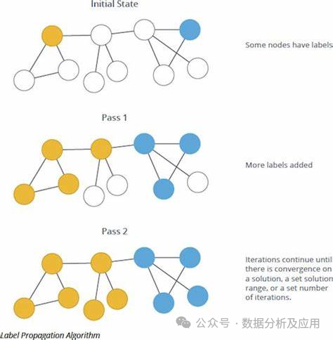
Label Propagation Algorithm

The label propagation algorithm is a graph-based semi-supervised learning method. Its basic principle is to iteratively update the label information of each node, gradually classifying unlabeled nodes into the categories of labeled nodes.

Model Principle:

The label propagation algorithm is a graph-based semi-supervised learning method that predicts the labels of unlabeled nodes using the label information of labeled nodes. Given a graph structure dataset containing both labeled and unlabeled nodes, the label propagation algorithm iteratively updates the label information of each node until convergence.

Model Training:

The training process involves the following steps:

1. Construct Graph Structure: Build a graph structure based on the relationships between samples in the dataset, where nodes represent samples, edges represent relationships between samples, and node labels represent sample label information.
2. Initialization: Set all unlabeled nodes to a temporary initial label.
3. Iterative Update: For each node, update its label information based on the label information of its neighbor nodes. Specifically, each node chooses the most frequently occurring label among its neighbor nodes as its new label and updates the label information of its neighbor nodes accordingly.
4. Convergence Check: Compare the label distributions before and after the iterative update. If the changes are small or a preset number of iterations is reached, stop the iteration; otherwise, return to step 3.

Advantages:

1. Simple Logic: The logic of the label propagation algorithm is straightforward and easy to understand and implement.
2. Low Time Complexity: The time complexity of the label propagation algorithm is O(n), where n is the number of nodes, thus exhibiting good performance when handling large-scale datasets.
3. Close to Linear Complexity: The complexity of the label propagation algorithm is linearly related to the number of nodes, resulting in excellent performance on large networks.
4. No Need to Define Optimization Function: The label propagation algorithm does not require defining an optimization function, thus avoiding complex gradient calculations and parameter tuning.
5. No Need to Predefine Community Counts: The label propagation algorithm uses its network structure to guide label propagation, eliminating the need to predefine community counts.

Disadvantages:

1. Avalanche Effect: Community results can be unstable and highly random. When the community labels of neighbor nodes have the same weight, a random choice may lead to a small initial error being amplified, resulting in an inappropriate outcome.
2. Asynchronous updates can lead to different community partition results based on the order of updates.

Usage Scenarios

Applicable to various scenarios requiring community discovery, such as social network analysis, image segmentation, recommendation systems, etc. It can partition datasets into communities with similar features, facilitating further analysis and mining. Additionally, it can also be used for anomaly detection and preprocessing in classification tasks. For example, in social network analysis, the label propagation algorithm can classify users into different communities and analyze the characteristics and behavior patterns of users in each community; in image segmentation, it can divide images into different regions or objects for feature extraction and analysis.

Example Code (Python)

The following Python code example uses label propagation to classify the iris flower:

from sklearn import datasets

from sklearn.semi_supervised import LabelSpreading

from sklearn.model_selection import train_test_split

from sklearn.metrics import classification_report, confusion_matrix

import numpy as np

import matplotlib.pyplot as plt

# Load dataset (using the iris dataset as an example)

iris = datasets.load_iris()

X = iris.data

y = iris.target

# Split the training and testing sets (using only 10% of labeled data for training)

X_train, X_test, y_train, y_test = train_test_split(X, y, test_size=0.2, random_state=42)

# Initialize model parameters (using default parameters here)

lp_model = LabelSpreading(kernel=’knn’, n_jobs=-1) # n_jobs=-1 means using all available CPU cores for computation

lp_model.fit(X_train, y_train) # Train the model on the training set

y_pred = lp_model.predict(X_test) # Predict on the test set

# Output classification result evaluation metrics (using classification report and confusion matrix)

print(confusion_matrix(y_test, y_pred)) # Output confusion matrix

print(classification_report(y_test, y_pred)) # Output classification report (including precision, recall, F1 score, etc.)

Conclusion

In summary, we systematically introduced machine learning models and their principles, where different machine learning models are suitable for different tasks and scenarios. This is because different machine learning models are based on different algorithms and principles, resulting in varying performance and characteristics when handling different types of data and problems.

For example, linear regression models are suitable for predicting continuous numerical data, while decision trees and random forests are suitable for classification and regression tasks. K-means clustering is suitable for clustering analysis in unsupervised learning, and PCA is suitable for data dimensionality reduction, feature extraction, and data visualization tasks.

Therefore, when selecting an appropriate machine learning model, it is necessary to choose based on the specific characteristics of the data and tasks. It is also important to consider the applicability and limitations of the model to avoid using certain models in unsuitable scenarios. Sometimes, it may be necessary to try different models and evaluate their performance through cross-validation to determine the most suitable model.

Editor: Wang Jing