This article will systematically and comprehensively introduce one of the commonly used frameworks in automated machine learning: Auto-Sklearn. It will cover installation and usage, classification and regression case studies, as well as some user manual introductions. Come and study with the little monkey!
AutoML
Automated Machine Learning (AutoML) is a relatively new field in machine learning that mainly automates all time-consuming processes in machine learning, such as data preprocessing, optimal algorithm selection, hyperparameter tuning, etc. This can save a lot of time in the process of building machine learning models.
Automated Machine Learning AutoML: For , let represent the feature vector, and represent the corresponding target value. Given the training dataset and the feature vector from the test dataset drawn from the same data distribution, along with resource budget and loss metrics , the AutoML problem is to automatically generate the predicted values for the test set, while gives the loss value of the solution to the AutoML problem.
AutoML is the process of discovering the best performance pipeline for data transformations, models, and model configurations for a dataset.
AutoML typically involves using complex optimization algorithms (such as Bayesian optimization) to effectively navigate the space of possible models and model configurations and quickly discover the most effective methods for a given predictive modeling task. It allows non-expert machine learning practitioners to quickly and easily discover effective or even optimal methods for a given dataset with little technical background or direct input.
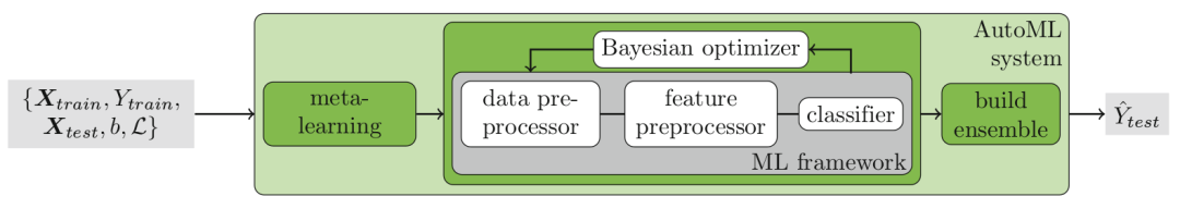
If you have used sklearn, you should find the above definition easy to understand. Let’s combine it with a flowchart for further understanding.
Auto-Sklearn
Auto-Sklearn is an open-source library for executing AutoML in Python. It leverages the popular Scikit-Learn machine learning library for data transformation and machine learning algorithms.
It was developed by Matthias Feurer and others, and described in their 2015 paper titled “Efficient and Robust Automated Machine Learning[1]“.
… we introduce a robust new AutoML system based on scikit-learn (using 15 classifiers, 14 feature preprocessing methods, and 4 data preprocessing methods, giving rise to a structured hypothesis space with 110 hyperparameters)
We introduce a robust new AutoML system based on scikit-learn (using 15 classifiers, 14 feature preprocessing methods, and 4 data preprocessing methods, resulting in a structured hypothesis space with 110 hyperparameters).
The benefit of Auto-Sklearn is that it not only discovers the data preprocessing and models to be executed for a dataset but also learns from models that perform well on similar datasets and can automatically create the best-performing ensemble as part of the optimization process.
This system, which we dub AUTO-SKLEARN, improves on existing AutoML methods by automatically taking into account past performance on similar datasets, and by constructing ensembles from the models evaluated during the optimization.
This system, which we call AUTO-SKLEARN, improves existing AutoML methods by automatically considering past performance on similar datasets and constructing ensembles from the models evaluated during optimization.
Auto-Sklearn improves upon general AutoML methods, using Bayesian hyperparameter optimization to effectively discover the optimal model pipeline for a given dataset.
Two additional components are added here:
- A meta-learning method for initializing the Bayesian optimizer
- An automated ensemble method during the optimization process
This meta-learning method complements Bayesian optimization for optimizing ML frameworks. For hyperparameter spaces as large as the entire ML framework, Bayesian optimization starts slowly. It selects several configurations based on meta-learning to seed the Bayesian optimization. This method can be referred to as a warm-start optimization method. Coupled with the automated ensemble method of multiple models, the entire machine learning process is highly automated, greatly saving users’ time. From this perspective, it allows machine learning users more time to select data and think about the problems themselves.
Bayesian Optimization
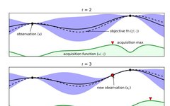
The principle of Bayesian optimization is to use the performance of existing samples in optimizing the objective function to build a posterior model. Each point on the posterior model is a Gaussian distribution, which has a mean and variance. If the point is an existing sample point, the mean is the value of the optimization objective function at that point, and the variance is 0. The mean and variance of other unknown sample points are fitted by posterior probability and may not be close to the real value. Therefore, an acquisition function is used to continuously probe the optimization objective function values corresponding to these unknown sample points, continuously updating the posterior probability model. Since the acquisition function can balance Explore/Exploit, it will tend to select points that perform well and have high potential. Thus, when resource budgets are exhausted, good optimization results can often be obtained, i.e., finding parameters in the local optimum of the optimization objective function.
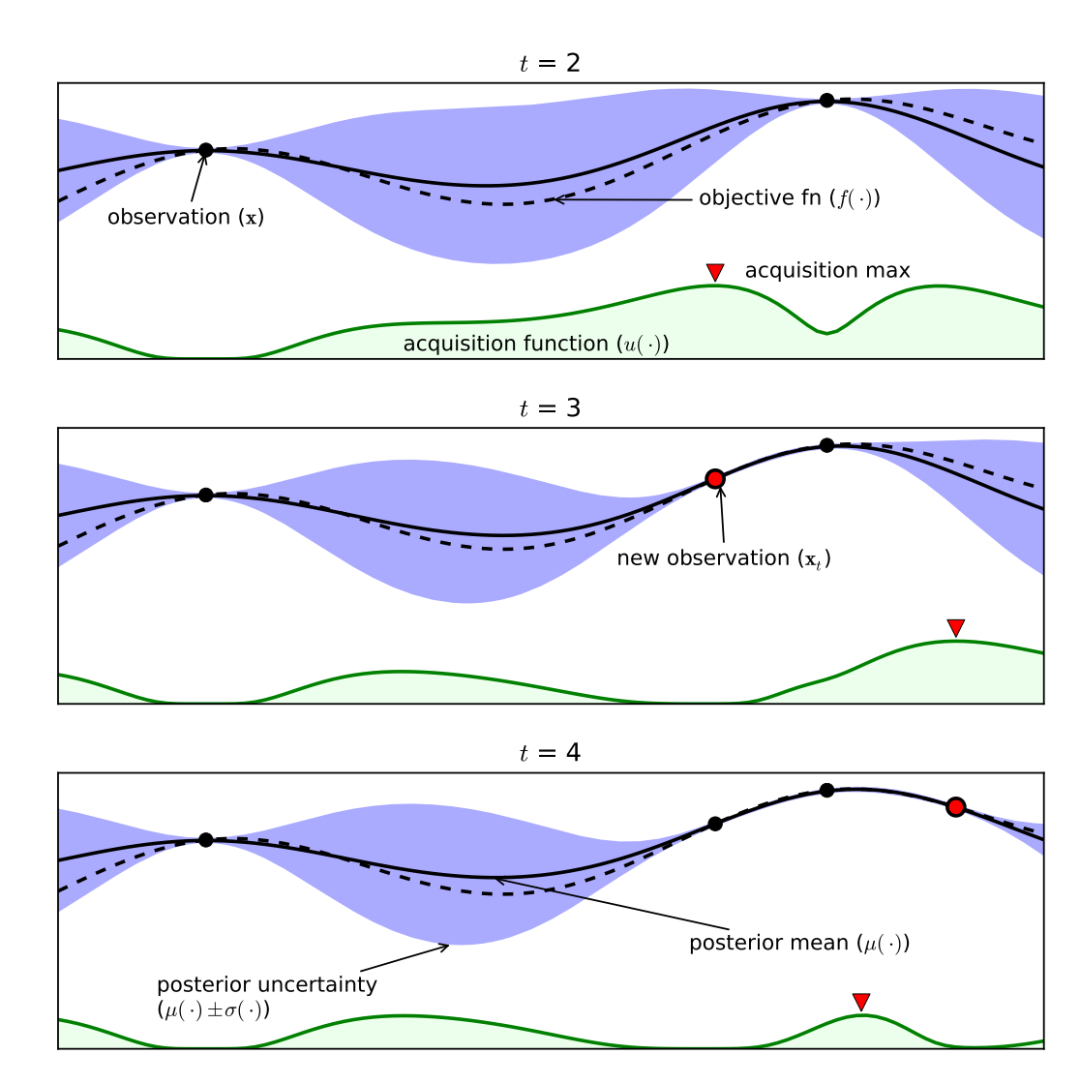
The above figure is an experimental graph applying Bayesian optimization to a simple 1D problem, showing the Gaussian process’s approximation of the objective function after four iterations. Taking t=3 as an example, we will explain the roles of various parts in the graph.
The above graph shows two evaluations with black dots and a red evaluation, which are the initial value estimates of the surrogate model after three evaluations, influencing the selection of the next point. There can be many curves drawn through these three points. The black dashed line curve is the actual true objective function (usually unknown). The black solid line curve is the mean of the surrogate model’s objective function. The purple area is the variance of the surrogate model’s objective function. The green shaded area indicates the value of the acquisition function, selecting the point with the maximum value as the next sampling point. With only three points, the fitting effect is slightly poor; the more black points there are, the smaller the area between the black solid line and the black dashed line, the smaller the error, and the closer the surrogate model is to the true model’s objective function.
Installing and Using Auto-Sklearn
Auto-sklearn provides out-of-the-box supervised automated machine learning. As the name suggests, auto-sklearn is built on the machine learning library scikit-learn and can automatically search for learning algorithms for new datasets and optimize their hyperparameters. Therefore, it frees machine learning users from tedious tasks, allowing them more time to focus on real problems.
Here, you can refer to the official documentation of auto-sklearn[2].
Ubuntu
>>> sudo apt-get install build-essential swig
>>> conda install gxx_linux-64 gcc_linux-64 swig
>>> curl `https://raw.githubusercontent.com/automl/auto-sklearn/master/requirements.txt` | xargs -n 1 -L 1 pip install
>>> pip install auto-sklearn
Anaconda
pip install auto-sklearn
After installation, we can import the library and print the version number to confirm it has been successfully installed:
# print autosklearn version
import autosklearn
print('autosklearn: %s' % autosklearn.__version__)
Your version number should be the same or higher.
autosklearn: 0.6.0
Depending on the predictive task, whether classification or regression, you can create and configure an instance of the AutoSklearnClassifier[3] or AutoSklearnRegressor[4] class and fit it to the dataset. That’s all. You can then use the generated model for direct predictions or save it to a file (using pickle) for later use.
AutoSklearn Class Parameters
The AutoSklearn class provides a wealth of configuration options as parameters.
By default, the search will use the train-test split of the dataset during the search process. For speed and simplicity, it is recommended to use the default values here.
The parameter n_jobs can be set to the number of cores in the system; for example, if there are 8 cores, set n_jobs=8.
Generally, the optimization process will run continuously and is measured in minutes. By default, it will run for one hour.
It is recommended to set the time_left_for_this_task parameter to the maximum time for this task (the desired seconds for the process to run). For many small predictive modeling tasks (datasets with fewer than 1,000 rows), less than 5-10 minutes may be sufficient. If nothing is specified for this parameter, the optimization process will continue to run for one hour, measured in minutes. In this case, the per_run_time_limit parameter is set to limit the time allocated for each model evaluation to 30 seconds. For example:
# define search
model = AutoSklearnClassifier(time_left_for_this_task=5*60,
                              per_run_time_limit=30,
                              n_jobs=8)
There are also other parameters like ensemble_size, initial_configurations_via_metalearning that can be used to fine-tune the classifier. By default, the above search command will create a set of the best-performing models. To avoid overfitting, we can disable it by changing the settings to ensemble_size = 1 and initial_configurations_via_metalearning = 0. We excluded these when setting up the classifier to keep the method simple.
At the end of the run, you can access the list of models and other details. The sprint_statistics() function summarizes the search and performance of the final model.
# summarize performance
print(model.sprint_statistics())
Classification Task
In this section, we will use Auto-Sklearn to discover models for the sonar dataset.
The sonar dataset[5] is a standard machine learning dataset consisting of 208 rows of data, 60 numerical input variables, and a target variable with two class values, such as binary classification.
Using a testing tool with three repetitions of stratified 10-fold cross-validation, a naive model can achieve about 53% accuracy. The best-performing model can achieve about 88% accuracy on the same testing tool. This provides the expected performance bounds for the dataset.
The dataset involves predicting whether sonar returns indicate rock or simulated mines.
# summarize the sonar dataset
from pandas import read_csv
# load dataset
dataframe = read_csv(data, header=None)
# split into input and output elements
data = dataframe.values
X, y = data[:, :-1], data[:, -1]
print(X.shape, y.shape)
Running this example will download the dataset and split it into input and output elements. You can see there are 60 input variables with 208 rows of data.
(208, 60) (208,)
First, split the dataset into training and testing sets, aiming to find a good model on the training set and then evaluate the performance of the found model on the holdout testing set.
# split into train and test sets
X_train, X_test, y_train, y_test = train_test_split(X, y, test_size=0.33, random_state=1)
Use the following command to import the classification model from autosklearn.
from autosklearn.classification import AutoSklearnClassifier
AutoSklearnClassifier is configured to run with 8 cores for 5 minutes and limits each model evaluation to 30 seconds.
# define search
model = AutoSklearnClassifier(time_left_for_this_task=5*60,
                              per_run_time_limit=30, n_jobs=8,
                              tmp_folder='/temp/autosklearn_classification_example_tmp')
Here, a temporary log saving path is provided, which we can use later to print the run details.
Then perform the search on the training dataset.
# perform the search
model.fit(X_train, y_train)
Report a summary of the search and the best-performing model.
# summarize
print(model.sprint_statistics())
You can print the leaderboard of all models considered for the search with the following command.
# leaderboard
print(model.leaderboard())
You can print information about the models considered with the following command.
print(model.show_models())
We can also apply techniques like SMOTE, ensemble learning (bagging, boosting), NearMiss algorithms, etc., to address the imbalance in the dataset.
Finally, evaluate the model’s performance on the testing dataset.
# evaluate best model
y_pred = model.predict(X_test)
acc = accuracy_score(y_test, y_pred)
print("Accuracy: %.3f" % acc)
You can also print the final ensemble score and confusion matrix.
# Score of the final ensemble
from sklearn.metrics import accuracy_score
m1_acc_score= accuracy_score(y_test, y_pred)
m1_acc_score
from sklearn.metrics import confusion_matrix, accuracy_score
y_pred= model.predict(X_test)
conf_matrix= confusion_matrix(y_pred, y_test)
sns.heatmap(conf_matrix, annot=True)
At the end of the run, a summary will be printed showing that 1,054 models were evaluated, with an estimated performance of the final model at 91%.
auto-sklearn results:
Dataset name: f4c282bd4b56d4db7e5f7fe1a6a8edeb
Metric: accuracy
Best validation score: 0.913043
Number of target algorithm runs: 1054
Number of successful target algorithm runs: 952
Number of crashed target algorithm runs: 94
Number of target algorithms that exceeded the time limit: 8
Number of target algorithms that exceeded the memory limit: 0
Then, evaluate the model on the holdout dataset, finding that the classification accuracy reached 81.2%, which is quite proficient.
Accuracy: 0.812
Regression Task
In this section, we will use Auto-Sklearn to mine models for the automobile insurance dataset.
The automobile insurance dataset[6] is a standard machine learning dataset consisting of 63 rows of data, one numerical input variable, and one numerical target variable.
Using a testing tool with three repetitions of stratified 10-fold cross-validation, a naive model can achieve an average absolute error (MAE) of about 66. The best-performing model can achieve about 28 MAE on the same testing tool. This provides the expected performance bounds for the dataset.
The dataset involves predicting the total claims amount (in thousands of Swedish Krona) based on the number of claims in different geographical areas.
You can use the same process as in the previous section, although we will use the AutoSklearnRegressor class instead of the AutoSklearnClassifier.
By default, the regressor will optimize the metric. If you need to use mean absolute error or MAE, you can specify it with the metric parameter when calling the fit() function.
# example of auto-sklearn for the insurance regression dataset
from pandas import read_csv
from sklearn.model_selection import train_test_split
from sklearn.metrics import mean_absolute_error
from autosklearn.regression import AutoSklearnRegressor
from autosklearn.metrics import mean_absolute_error as auto_mean_absolute_error
# load dataset
dataframe = read_csv(data, header=None)
# split into input and output elements
data = dataframe.values
data = data.astype('float32')
X, y = data[:, :-1], data[:, -1]
# split into train and test sets
X_train, X_test, y_train, y_test = train_test_split(X, y,
                                                    test_size=0.33,
                                                    random_state=1)
# define search
model = AutoSklearnRegressor(time_left_for_this_task=5*60,
                             per_run_time_limit=30, n_jobs=8)
# perform the search
model.fit(X_train, y_train, metric=auto_mean_absolute_error)
# summarize
print(model.sprint_statistics())
# evaluate best model
y_hat = model.predict(X_test)
mae = mean_absolute_error(y_test, y_hat)
print("MAE: %.3f" % mae)
At the end of the run, a summary will be printed showing that 1,759 models were evaluated, with an estimated performance of the final model at 29 MAE.
auto-sklearn results:
Dataset name: ff51291d93f33237099d48c48ee0f9ad
Metric: mean_absolute_error
Best validation score: 29.911203
Number of target algorithm runs: 1759
Number of successful target algorithm runs: 1362
Number of crashed target algorithm runs: 394
Number of target algorithms that exceeded the time limit: 3
Number of target algorithms that exceeded the memory limit: 0
Saving Trained Models
The classification and regression models trained above can be saved using the Python packages Pickle and JobLib. These saved models can then be used directly for predictions on new data. We can save the model as:
1. Pickle
import pickle
# save the model
filename = 'final_model.sav'
pickle.dump(model, open(filename, 'wb'))
The “wb” parameter here means we are writing the file to disk in binary mode. Additionally, we can load this saved model as:
#load the model
loaded_model = pickle.load(open(filename, 'rb'))
result = loaded_model.score(X_test, Y_test)
print(result)
The “rb” command here indicates we are reading the file in binary mode.
2. JobLib
Similarly, we can save the trained model in JobLib with the following command.
import joblib
# save the model
filename = 'final_model.sav'
joblib.dump(model, filename)
We can also reload these saved models later to predict new data.
# load the model from disk
load_model = joblib.load(filename)
result = load_model.score(X_test, Y_test)
print(result)
User Manual Address
Below we will interpret the user manual[7] from several aspects.
Time and Memory Limits
A key feature of auto-sklearn is to limit the resources (memory and time) that scikit-learn algorithms can use. Especially for large datasets (where algorithms may take hours and engage in machine swapping), it is important to stop evaluations after a certain period to make progress within a reasonable time. Therefore, setting resource limits is a trade-off between optimizing time and the number of models that can be tested.
Although auto-sklearn alleviates the speed of manual hyperparameter tuning, users still need to set memory and time limits. For most datasets, a memory limit of 3GB or 6GB on most modern computers is sufficient. For time limits, it is difficult to give clear guidelines. If possible, a good default is a total limit of one day, with a single run limit of 30 minutes.
More guidelines can be found at auto-sklearn/issues/142[8].
Limiting the Search Space
In addition to using all available estimators, you can limit the search space of auto-sklearn. The example below shows how to exclude all preprocessing methods and limit the configuration space to only use random forests.
import autosklearn.classification

automl = autosklearn.classification.AutoSklearnClassifier(
    include_estimators=["random_forest",],
   exclude_estimators=None,
    include_preprocessors=["no_preprocessing", ],
    exclude_preprocessors=None)

automl.fit(X_train, y_train)
predictions = automl.predict(X_test)
Note: The strings used to identify estimators and preprocessors are the file names without .py.
Turning Off Preprocessing
Preprocessing in auto-sklearn is divided into data preprocessing and feature preprocessing. Data preprocessing includes one-hot encoding for categorical features, missing value imputation, and normalization of features or samples. These steps cannot currently be turned off. Feature preprocessing consists of individual feature transformers that implement tasks such as feature selection or transforming features to different spaces (like PCA). As shown in the example above, feature preprocessing can be turned off by setting include_preprocessors=["no_preprocessing"].
Resampling Strategies
Examples using maintained datasets and cross-validation can be found in auto-sklearn/examples/.
Result Checking
Auto-sklearn allows users to check the training results and view relevant statistics. The following example shows how to print different statistics for corresponding checks.
import autosklearn.classification

automl = autosklearn.classification.AutoSklearnClassifier()
automl.fit(X_train, y_train)
automl.cv_results_
automl.sprint_statistics()
automl.show_models()
cv_results_returns a dictionary where the keys serve as column headers, and the values as columns, which can be imported into aDataFrametype data inpandas.sprint_statistics()can print the dataset name, the metric used, and the best validation score achieved through runningauto-sklearn. Additionally, it prints the number of successful and unsuccessful algorithm runs.- By calling
show_models(), you can print the results produced by the final ensemble model.
Parallel Computing
Auto-sklearn supports parallel execution by sharing data on a shared file system. In this mode, the SMAC algorithm shares its training data by writing it to disk after each iteration. At the start of each iteration, SMAC loads all newly discovered data points. We provide an example that implements the n_jobs feature of scikit-learn and a guide on how to manually start multiple auto-sklearn instances.
In default mode, auto-sklearn uses two cores. The first is for model building, and the second is used to build the ensemble after each new machine learning model finishes training. The sequential example shows how to run these tasks sequentially using only one core at a time.
Additionally, depending on the installation of scikit-learn and numpy, the model building process can utilize all cores at once. This behavior is not desired by auto-sklearn and is likely due to numpy being installed as a binary wheel from pypi (see here). Executing export OPENBLAS_NUM_THREADS=1 should disable this behavior and ensure that numpy uses only one core at a time.
Vanilla Auto-Sklearn
Auto-sklearn is primarily a wrapper based on scikit-learn. Therefore, persistence examples in scikit-learn can be followed.
To obtain the vanilla auto-sklearn used in the materials Efficient and Robust Automated Machine Learning, set ensemble_size = 1 and initial_configurations_via_metalearning=0.
import autosklearn.classification
automl = autosklearn.classification.AutoSklearnClassifier(
    ensemble_size=1, initial_configurations_via_metalearning=0)
Setting the ensemble size to 1 will result in always selecting the single model with the best test performance on the validation set. Setting the initial configurations via meta-learning to 0 will make auto-sklearn use the standard SMAC algorithm to set new hyperparameter configurations.
References
[1]
Efficient and Robust Automated Machine Learning: https://papers.nips.cc/paper/5872-efficient-and-robust-automated-machine-learning
[2]
Official Documentation of Auto-Sklearn: https://automl.github.io/auto-sklearn/master/installation.html
[3]
AutoSklearnClassifier: https://automl.github.io/auto-sklearn/master/api.html#classification
[4]
AutoSklearnRegressor: https://automl.github.io/auto-sklearn/master/api.html#regression
[5]
Sonar Dataset: https://gitee.com/yunduodatastudio/picture/raw/master/data/auto-sklearn.png
[6]
Automobile Insurance Dataset: https://gitee.com/yunduodatastudio/picture/raw/master/data/auto-sklearn.png
[7]
User Manual: https://automl.github.io/auto-sklearn/master/manual.html#manual
[8]
Auto-sklearn/issues/142: https://github.com/automl/auto-sklearn/issues/142
[9]
https://cloud.tencent.com/developer/article/1630703
[10]
https://machinelearningmastery.com/auto-sklearn-for-automated-machine-learning-in-python/