Follow the public account “ML_NLP“
Set as “Starred“, heavy content delivered first!

Reprinted from | PaperWeekly
©PaperWeekly Original · Author|Sun Yudao
School|PhD student at Beijing University of Posts and Telecommunications
Research Direction|GAN Image Generation, Emotion Adversarial Sample Generation

A Mathematical Introduction to Generative Adversarial Nets
https://arxiv.org/abs/2009.00169
Introduction
Since the pioneering work of Goodfellow on GANs in 2014, GANs have garnered significant attention, leading to an explosive growth of new ideas, technologies, and applications.
The original paper on GANs contains some rigorous proofs, and for training efficiency, many simplifications have been made. This is actually a common phenomenon in the field. In a summer course on the mathematical principles of deep learning at Peking University, the instructor mentioned that mathematical rigor accounts for 60% in deep learning.
The implication is that the proof processes in this field are not as rigorous as pure mathematics. When deriving proofs from the perspective of a computer science engineer, there are often premise assumptions that contradict practical realities; however, the conclusions derived from these assumptions often align with experimental results or provide some guidance for solving practical problems.
The author is a mathematically proficient AI researcher. The purpose of this paper is to provide an overview of GANs from a mathematical perspective, making it a rare theoretical article on the mathematical principles of GANs. The paper involves a considerable amount of mathematical principles and many dazzling mathematical symbols, which can be regarded as a theoretical manual for GANs, allowing readers to study the sections they are interested in in depth.
Background of GANs
The Turing Award winner Yann LeCun, known as one of the three musketeers of deep learning, once stated, “The introduction of GANs is the most interesting idea in deep learning in the last decade.”
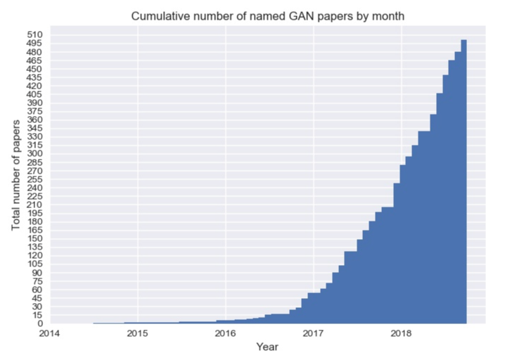
The following figure shows the number of papers published monthly on GANs from 2014 to 2018. It can be seen that after the introduction of GANs in 2014, there were relatively few related papers until 2016. However, from 2016 or 2017 to this year, there has indeed been an explosive growth in related papers.
GANs have a wide range of applications, including image synthesis, image editing, style transfer, image super-resolution, image transformation, data augmentation, and more.
In this paper, the author will attempt to introduce GANs from a more mathematical perspective for beginners. To fully understand GANs, one must also study their algorithms and applications, but understanding the mathematical principles is the key first step to grasping GANs. With this understanding, mastering other variants of GANs will become easier.
The goal of GANs is to solve the following problem: Suppose there is a dataset of objects, such as a set of cat images, handwritten Chinese characters, or paintings by Van Gogh. GANs can generate similar objects from noise, with the principle that neural networks appropriately adjust network parameters using the training dataset, and deep neural networks can approximate any function.
For the discriminator function D and the generator function G modeled as neural networks, the specific model of GANs is shown in the figure below. The GAN network actually consists of two networks: one is the generator network G used to generate fake samples, and the other is the discriminator network D used to distinguish between real and fake samples. To introduce adversarial loss, the generator is trained in a way that enables it to produce high-quality images through adversarial training.

Specifically, adversarial learning can be achieved through the maximization-minimization of the objective function between the discriminator function and the generator function. The generator G transforms random samples from distribution into generated samples. The discriminator attempts to distinguish them from real samples from the distribution, while G tries to make the generated samples similar to the training samples in distribution.
Mathematical Formulas of GANs
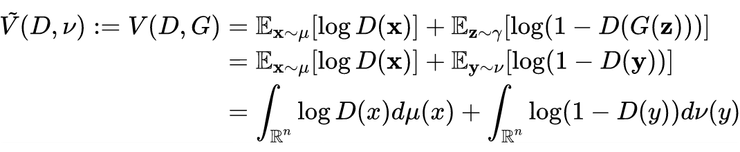
The adversarial game of GANs can be mathematically represented by the maximization-minimization of the objective function between the discriminator function and the generator function. The generator transforms random samples from distribution into generated samples. The discriminator attempts to distinguish them from training samples from the distribution, while tries to make the generated samples similar to the training samples in distribution. The adversarial loss function is as follows:

In the formula, the expectation is indicated by the specified distribution in the subscript. The description of the minimax value solved by GAN is as follows:

Intuitively, for a given generator, optimizing the discriminator to distinguish the generated samples means trying to assign high values to real samples from the distribution and low values to generated samples.
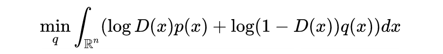
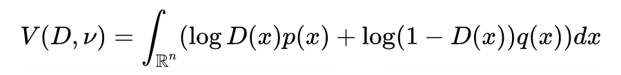
Conversely, for a given discriminator, optimizing the generator will attempt to “fool” the discriminator into assigning high values.Let be the distribution, which can be rewritten as and as:
Transform the above maximization-minimization problem into the following formula:

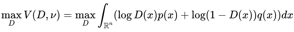
Assuming that has density , and has density function (it is important to note that this only occurs when ). In summary, it can finally be written as:
It can be observed that under certain constraints of , the above value is equivalent to .
The paper contains a large number of formulas and proofs, which can be quite overwhelming. Different propositions and theorems appear interspersed, so to reduce reading barriers for readers, I have selected some propositions and theorems that I consider important and reorganized them.
Proposition 1: Given probability distributions and on , with their probability density functions being and , the following holds:
Where , the range of values is (sup represents the supremum).
Theorem 1: Let be a probability density function on . For the probability distributions with density functions and , the maximization-minimization problem can be described as:

For all , it can be solved that and .
Theorem 1 states that the solution to the maximization-minimization problem is the optimization solution of GAN derived by Ian Goodfellow in that 2014 paper.
Theorem 2: Let be a given probability distribution on . For probability distributions and function , the following holds:

Where and exist almost everywhere for .
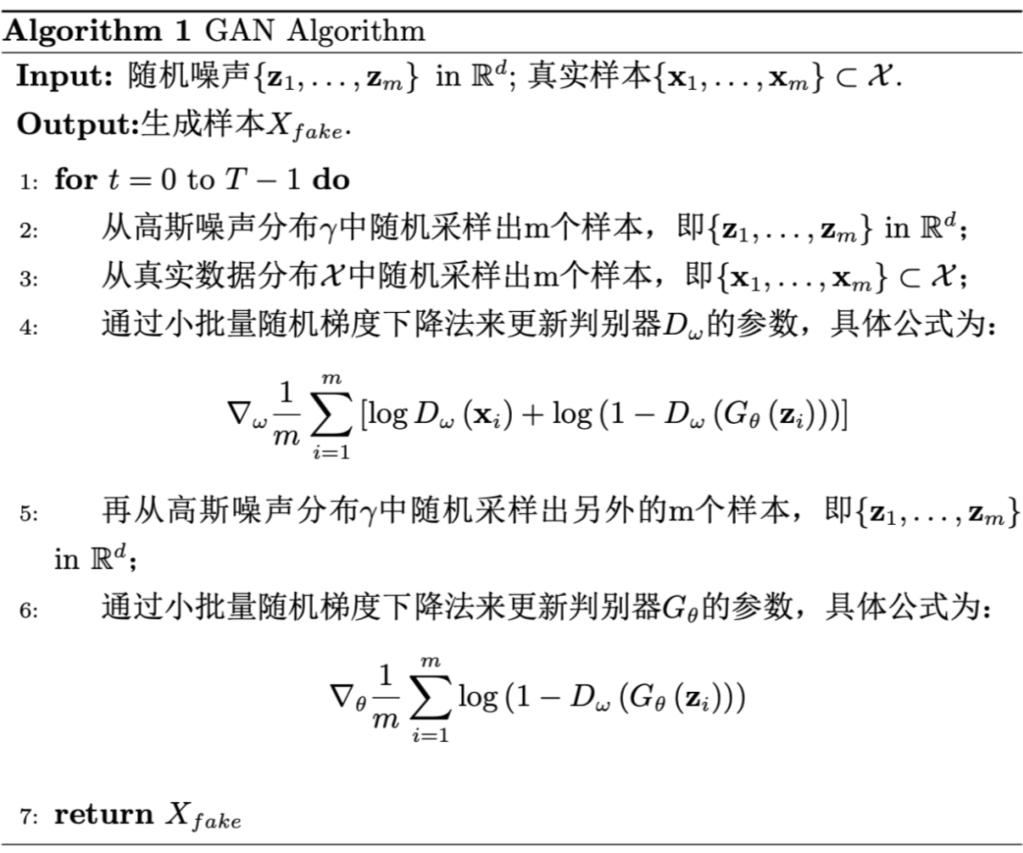
Proposition 2: If the discriminator is allowed to reach its best given in each training cycle, then updating according to the minimization criterion yields:
Where the distribution converges to the distribution .
From a purely mathematical perspective, Proposition 2 is not rigorous. However, it provides a practical framework for solving the minimax problem of GANs.
In summary, the propositions and theorems can be summarized into the following GAN algorithm framework. For clarity, I have reorganized this algorithm framework.
f-Divergence and f-GAN
4.1 f-Divergence
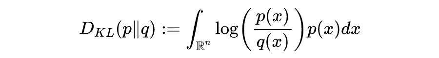
The essence of GANs is to bring the distribution of random noise closer to the real data distribution through adversarial training, which requires a metric to measure probability distributions—divergence. The well-known KL divergence formula is as follows (KL divergence has a drawback of distance asymmetry, so it is not a true distance metric in the traditional sense).
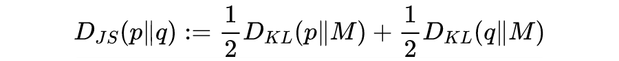
And the JS divergence formula is as follows (JS divergence improves upon the distance asymmetry of KL divergence):
However, all the divergences we are familiar with can be summarized into a larger category known as f-divergence, defined as follows:
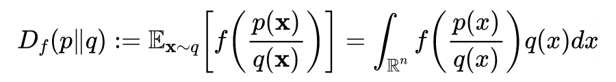
Definition 1: Let and be two probability density functions on . The f-divergence between and is defined as:
Where, if is true, then .
It is important to understand that the f-divergence varies depending on the chosen function, leading to different degrees of asymmetry in distance.
Proposition 3: Let be a strictly convex function on the domain , such that . Assume (equivalent to ) or , where . Then , if and only if .
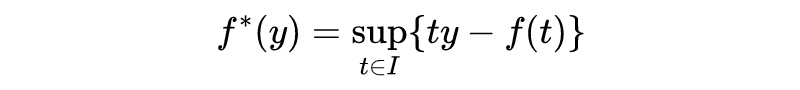
4.2 Convex Functions and Convex Conjugates
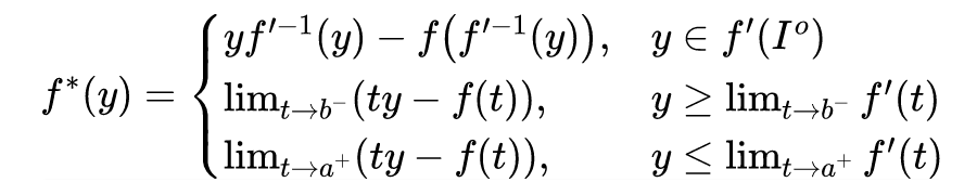
The convex conjugate of a convex function is also known as the Fenchel transform or Fenchel-Legendre transform, which is a generalization of the well-known Legendre transform. Let be a convex function defined on the interval . Its convex conjugate is defined as:
Lemma 1: Assume is strictly convex and continuously differentiable on its domain , where . Then:
Proposition 4: Let be a convex function on . Its range is within . Then is convex and lower semi-continuous. Moreover, if is lower semi-continuous, then it satisfies the Fenchel duality.
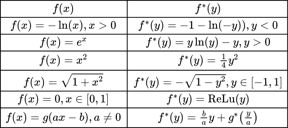
The table below lists some common convex functions and their convex duals:
4.3 Estimating f-Divergence Using Convex Duality
To estimate the f-divergence of samples, the convex dual of f can be used. The derivation formula is as follows:
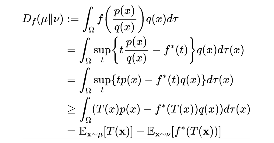
Where is any Borel function, thus obtaining all Borel functions as follows:
Proposition 5: Let be strictly convex and continuously differentiable on . Let , be Borel probability measures on , such that . Then:

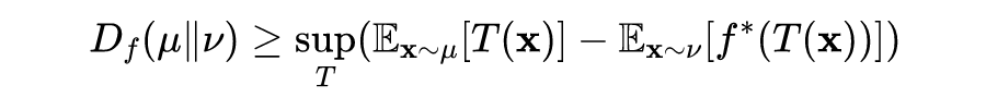
Theorem 3: Let be convex, such that the domain of contains certain . Let be Borel probability measures on , then:

Where for all Borel functions, .
Theorem 4: Let be a lower semi-continuous convex function, such that the domain of has . Let be Borel probability measures on , such that , where and . Then:
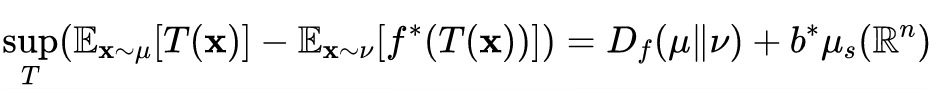
Where for all Borel functions, .
4.4 f-GAN and VDM
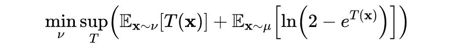
Using f-divergence to represent the generalization of GAN. For a given probability distribution, the goal of f-GAN is to minimize the f-divergence with respect to the probability distribution. In the sample space, f-GAN solves the following maximization-minimization problem:
This optimization problem can be referred to as Variational Divergence Minimization (VDM). Note that VDM appears similar to the maximization-minimization problem in GAN, where the Borel function is referred to as the judging function.
Theorem 5: Let be a lower semi-continuous strictly convex function, such that the domain of is . Further assume that is continuously differentiable on its domain, and . Let be Borel probability measures on , then:
Where for all Borel functions, .
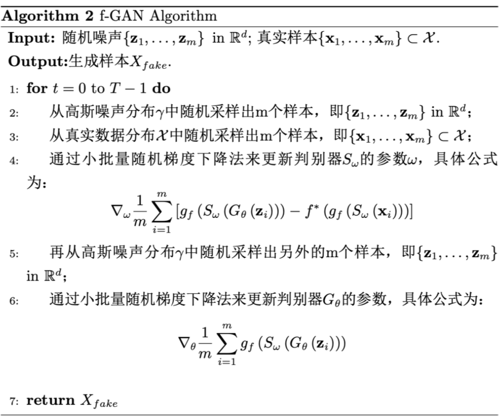
In summary, below is the algorithm process framework for f-GAN.
4.4.1 Example1:
When the function , the f-divergence here is the familiar KL divergence. Its conjugate function is , where , and its corresponding objective function is:

Where , ignoring the constant +1 term, and , will lead to the original form of GAN:
4.4.2 Example2:
This is the Jensen-Shannon divergence, whose conjugate function is , domain . The corresponding f-GAN objective function is:
Where , , so it can be further simplified to:

Where the constant term is ignored in this formula.
4.4.3 Example3: ,
The conjugate function of this function is , domain . When is not strictly convex and continuously differentiable, the corresponding f-GAN objective function is as follows:

The form of this objective function is the objective function of Wasserstein GAN.
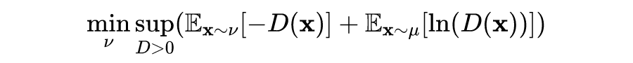
4.4.4 Example4:
Given , this function is strictly convex. The corresponding f-GAN objective function is:

Further solving the above formula yields:
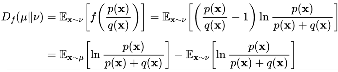
In this formula, the “logD” technique used in the original GAN paper is included to address the gradient saturation problem in GANs.
Specific Examples of GANs
For the application examples of GANs, I have not introduced the examples given in the paper; instead, I introduced the GANs that I personally find interesting.
Training a GAN can be challenging, often encountering various issues, the main three being:
-
Vanishing Gradient: This often occurs, especially when the discriminator is too good, hindering the improvement of the generator. When using the optimal discriminator, training may fail due to vanishing gradients, failing to provide sufficient information for the generator to improve.
-
Mode Collapse: This refers to the phenomenon where the generator starts to repeatedly produce the same output (or a small group of outputs). If the discriminator gets stuck in a local minimum, the next generator iteration can easily find the most reasonable output for the discriminator. The discriminator can never learn to escape this trap.
-
Failure to Converge: Due to many known and unknown factors, GANs often fail to converge.
WGAN makes a simple modification by replacing the Jensen-Shannon divergence loss function in GAN with the Wasserstein distance (also known as Earth Mover’s distance). Do not underestimate the significance of this modification: it is one of the most important advancements since the birth of GANs, as the use of Wasserstein distance effectively addresses some prominent shortcomings of divergence-based GANs, thereby alleviating common failure modes in GAN training.
DCGAN introduces convolutions into the training process of GANs, improving the parameter count and training effects. It provides many guiding directions in training GANs, specifically including the following five points:
-
Replace any pooling layers in the generator and discriminator with strided convolutions.
-
Use batch normalization in both the generator and discriminator.
-
Remove fully connected hidden layers to achieve a deeper architecture.
-
In addition to using Tanh as the output, use ReLU activation for all layers in the generator.
-
Use LeakyReLU activation in the discriminator across all layers.
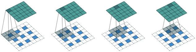
It is important to note that the discriminator processes from high-dimensional vectors to low-dimensional vectors through a convolution process, as shown in the following image:

The generator processes from low-dimensional vectors to high-dimensional vectors through a deconvolution process, also known as transposed convolution and fractional stride convolution. The difference between convolution and deconvolution lies in the padding method, as can be seen in the image below:
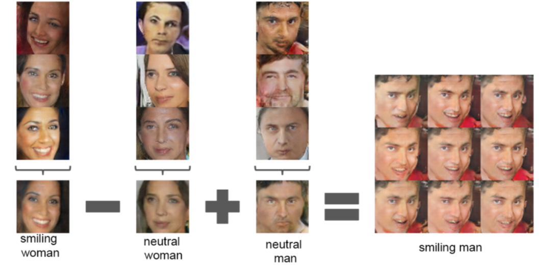
Another important innovation of DCGAN is the introduction of vector addition into image generation, as shown in the following image:
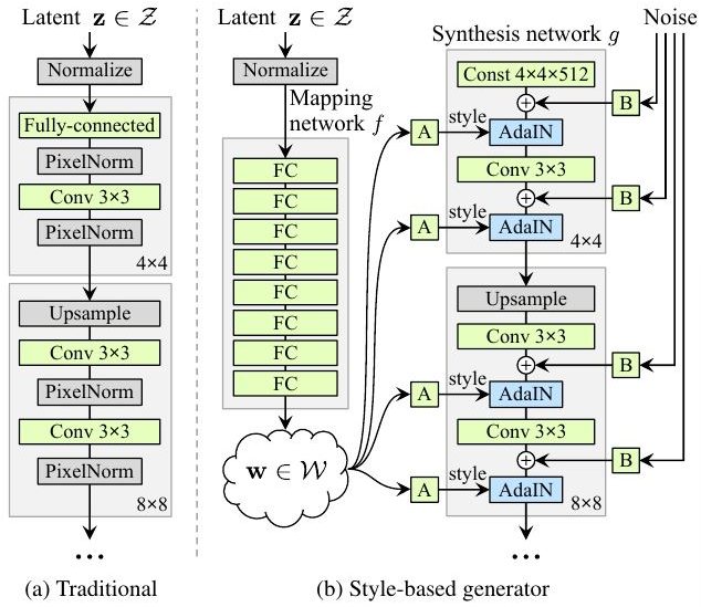
5.3 StyleGAN
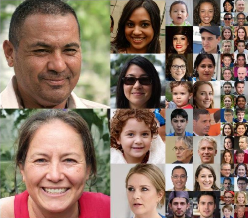
StyleGAN proposes a new generator framework that claims to control high-level attributes of the generated images, such as hairstyle, freckles, etc. The generated images score better on some evaluation metrics. As a type of unsupervised learning GAN, it can generate high-resolution images from noise. The specific algorithm framework diagram is shown below:
The clarity and detail of the images generated by StyleGAN can be seen in the following image, though the training cost is also quite high.
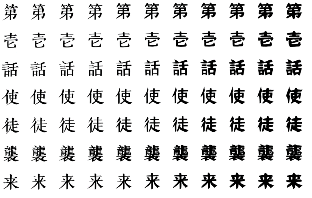
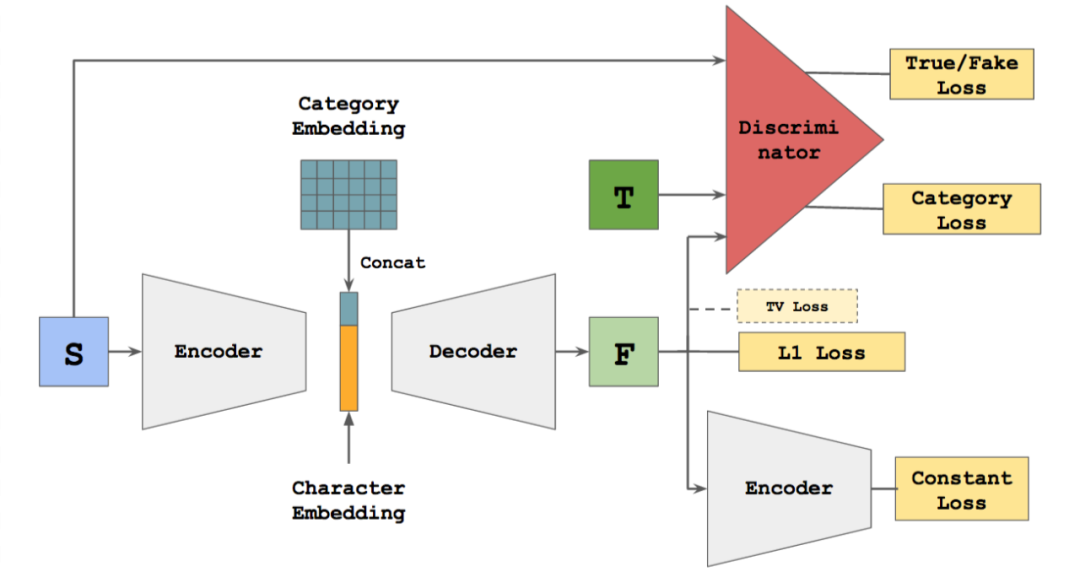
5.4 zi2zi
zi2zi is one of my favorite applications of GANs, utilizing GANs to transform font styles. Previous work dealt with similar Chinese font transformation issues, but the results were not ideal. The reasons include that the generated images are often blurry, and when processing more stylistic fonts, the effects are poor, as each time it could only learn and output a limited target font style. GANs can effectively solve these problems, with the model framework shown in the figure below:
Chinese characters, whether simplified or traditional, or Japanese characters, are constructed using the same principles and have a series of common foundations. The specific implementation results are shown in the figure below: