Comprehensive Explanation of Gaussian Mixture Model (GMM)

Hello everyone~

Today we are going to talk about a probabilistic model – Gaussian Mixture Model (GMM).

Gaussian Mixture Model is like a complex fuzzy grouping mechanism, believing that a dataset is actually composed of multiple “small groups,” where things within each “small group” are roughly distributed according to a bell curve (Gaussian distribution). You can imagine it as several overlapping bell curves that together form the whole of the data you see.

Gaussian Mixture Model is a probabilistic model used to represent a dataset composed of multiple Gaussian distributions (normal distributions). GMM assumes that each data point in the dataset is generated by one of several underlying Gaussian distributions. The parameters of these Gaussian distributions (such as mean and variance) and their weights (the contribution of each distribution) need to be estimated.

Mathematically, the form of GMM can be expressed as:

Where:

• is the data point.
• is the number of Gaussian distributions (also known as components).
• is the mixing weight of the k-th Gaussian distribution, satisfying .
• is the k-th Gaussian distribution, with mean and covariance matrix .

To think of a very intuitive example, you can imagine~

Suppose you measured the heights of people in different coffee shops around the city. Due to the different height distributions of people in different regions, you would find that the data you measured has several distinct “peaks,” each representing a height distribution of a region. If these peaks are viewed as individual Gaussian distributions (bell curves), then GMM will tell you which bell curve generated each data point (each person’s height), or in other words, to which “group” it belongs.

Theoretical Basis

The Gaussian Mixture Model (GMM) is a probabilistic model based on statistics, used to represent a dataset composed of multiple Gaussian distributions.

The core idea is to assume that the data is generated by a mixture of several different Gaussian distributions.

1. Gaussian Distribution

The Gaussian distribution, also known as the normal distribution, is a continuous probability distribution with a bell-shaped curve. For a d-dimensional data point , its probability density function (pdf) is defined as:

Where, is the mean vector, is the covariance matrix, and is the determinant of the covariance matrix.

1. Gaussian Mixture Model (GMM)

GMM assumes that the data point is generated by a weighted combination of K Gaussian distributions, and its probability density function is a linear combination of these Gaussian distributions:

Where, is the mixing weight of the k-th Gaussian distribution, satisfying , and and are the mean and covariance matrix of the k-th Gaussian distribution respectively.

1. Expectation-Maximization (EM) Algorithm

The EM algorithm is used to estimate the parameters of GMM, including the mean vector , covariance matrix , and mixing weights . It gradually optimizes these parameters by alternately executing two steps: the Expectation step (E-step) and the Maximization step (M-step).

Algorithm Flow

The learning process of the Gaussian Mixture Model is usually implemented through the EM algorithm.

1. Initialization

Select initial parameters :

• Mean vector
• Covariance matrix
• Mixing weights

The initialization method can be random initialization or based on other methods (e.g., K-means results).

1. Expectation Step (E-step)

Calculate the posterior probability of each data point belonging to each Gaussian distribution, i.e., the responsibility, which indicates the probability that the k-th data point is generated by the k-th Gaussian distribution. Its formula is:

Where, is the k-th data point, indicating the probability that data point belongs to the k-th Gaussian distribution.

1. Maximization Step (M-step)

Use the posterior probabilities obtained from the E-step to update the parameters. The new parameters are obtained by maximizing the log-likelihood estimate:

• Update mixing weights:

Where, indicates the total responsibility of all data points for the k-th Gaussian distribution, and is the total number of data points.

• Update mean vector:

• Update covariance matrix:

1. Check Convergence

Check whether the changes in parameters or the changes in log-likelihood meet the preset convergence conditions (e.g., less than a certain threshold). If the convergence conditions are met, stop the iteration; otherwise, return to the E-step.

1. Output Results

When the convergence conditions are met, output the estimated parameters.

An Example

Suppose we have a two-dimensional dataset and believe it is generated by two Gaussian distributions:

1. Initialization:

• Randomly select two initial means, e.g., and .
• Initialize covariance matrix, e.g., (identity matrix).
• Initialize mixing weights to be equal, e.g., .

1. Expectation Step (E-step):

• Calculate the responsibility (posterior probability) for each data point belonging to each Gaussian distribution.

1. Maximization Step (M-step):

• Use the responsibilities to update the means, covariance matrices, and mixing weights.

1. Check Convergence:

• Check if parameters have converged, if not, repeat E-step and M-step.

Finally, obtain the parameters of the two Gaussian distributions, which together describe the distribution of the data. Through these parameters, one can understand how the data is generated by these two distributions.

Application Scenarios

The Gaussian Mixture Model (GMM) is suitable for the following types of problems:

1. Clustering

   GMM is used to divide a dataset into multiple clusters, each described by a Gaussian distribution. Compared to K-means clustering, GMM allows clusters to have different shapes, sizes, and orientations.

2. Density Estimation

   GMM can be used to estimate the probability density function of the data, suitable for scenarios requiring estimation of complex distributions. For example, for generating new data points or making probability predictions.

3. Anomaly Detection

   By estimating the probability density of the data, low-probability data points can be identified, suitable for detecting anomalies or abnormal behaviors. For example, identifying anomalous traffic in cybersecurity.

4. Data Generation

   Using GMM to generate new data points similar to the original data, suitable for tasks such as synthetic data generation and data augmentation.

Advantages and Disadvantages

Advantages:

1. Flexibility: GMM can handle complex multimodal data distributions, allowing different means and covariance matrices for each Gaussian component.
2. Soft Assignment: Unlike K-means, GMM assigns probabilities to each data point rather than hard assignments, making this soft assignment suitable for handling overlapping clusters.
3. Probabilistic Interpretation: GMM provides a probabilistic interpretation, suitable for applications requiring probability outputs.
4. Density Estimation: Capable of estimating the probability density of data, suitable for data with unknown distributions.

Disadvantages:

1. Sensitive to Initial Values: GMM is sensitive to initial parameters, and different initializations may lead to different results.
2. May Get Stuck in Local Optima: The EM algorithm may converge to local optima, requiring multiple runs to avoid this.
3. Computational Complexity: Especially for high-dimensional or large-scale data, calculating the covariance matrix and probability density can be very complex.
4. Assumes Data is Gaussian Distributed: If the data significantly deviates from the Gaussian distribution assumption, GMM may perform poorly.

Prerequisites for Application

1. Data Independent and Identically Distributed: Assumes that data points are independent and identically distributed.
2. Cluster Structure Can Be Represented as Gaussian Distribution: Assumes that each cluster can be described by a Gaussian distribution, meaning the clusters of data are elliptical distributions.
3. Parameter Initialization: Reasonable parameter initialization is needed to improve the probability of converging to a global optimum.
4. Moderate Dimensions: For very high-dimensional data, calculating the covariance matrix may be complex and may require dimensionality reduction.

Complete Case Study

Now we will use Python to perform GMM clustering on a large-scale dataset and demonstrate how to optimize the algorithm and visualize complex results. Through this case study, everyone can basically understand the logic behind it.

Here we take a synthetic large dataset as an example.

1. Set Up Environment and Import Libraries

For libraries you are not familiar with, you can look them up individually to understand their functions.

import numpy as np
import pandas as pd
import matplotlib.pyplot as plt
from mpl_toolkits.mplot3d import Axes3D
from sklearn.mixture import GaussianMixture
from sklearn.preprocessing import StandardScaler
from sklearn.decomposition import PCA
from sklearn.datasets import make_blobs
from scipy.spatial.distance import cdist

2. Create Synthetic Dataset

Generate a synthetic three-dimensional large dataset to simulate complex Gaussian mixture distribution data.

# Set seed for reproducibility
np.random.seed(42)

# Generate synthetic dataset
n_samples = 100000
n_features = 3
n_clusters = 5

X, true_labels = make_blobs(n_samples=n_samples, n_features=n_features, centers=n_clusters, cluster_std=1.5, random_state=42)

# Standardize data
scaler = StandardScaler()
X_scaled = scaler.fit_transform(X)

# Convert data to DataFrame
df = pd.DataFrame(X_scaled, columns=['Feature1', 'Feature2', 'Feature3'])

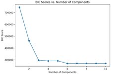
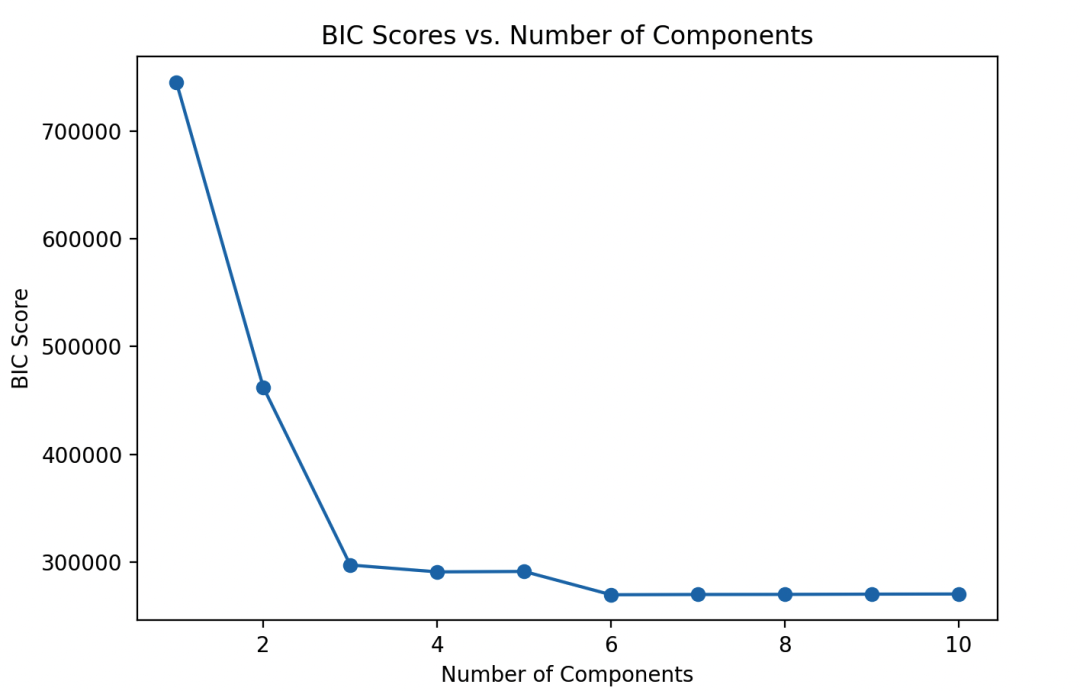
3. Determine the Optimal Number of Clusters

Use the elbow method to determine the optimal number of components for GMM.

# Range from 1 to 10
n_components_range = range(1, 11)

# Save BIC values
bic_scores = []

for n_components in n_components_range:
    gmm = GaussianMixture(n_components=n_components, random_state=42)
    gmm.fit(X_scaled)
    bic_scores.append(gmm.bic(X_scaled))

# Plot BIC values
plt.plot(n_components_range, bic_scores, marker='o')
plt.title('BIC Scores vs. Number of Components')
plt.xlabel('Number of Components')
plt.ylabel('BIC Score')
plt.show()

# Print optimal number of components
best_n_components = np.argmin(bic_scores) + 1
print(f'Optimal number of components: {best_n_components}')

4. Apply GMM for Clustering

Train the GMM model using the optimal number of components and predict the cluster labels for data points.

# Train GMM
gmm = GaussianMixture(n_components=best_n_components, covariance_type='full', random_state=42)
gmm.fit(X_scaled)
labels = gmm.predict(X_scaled)

# Add labels to DataFrame
df['Cluster'] = labels

5. Visualize Results

Use a 3D scatter plot and Principal Component Analysis (PCA) to visualize the clustering results of high-dimensional data.

# 3D visualization
fig = plt.figure(figsize=(10, 8))
ax = fig.add_subplot(111, projection='3d')
scatter = ax.scatter(df['Feature1'], df['Feature2'], df['Feature3'], c=labels, cmap='viridis', alpha=0.5)
legend1 = ax.legend(*scatter.legend_elements(), title="Clusters")
ax.add_artist(legend1)
ax.set_title('3D Scatter Plot of GMM Clusters')
ax.set_xlabel('Feature1')
ax.set_ylabel('Feature2')
ax.set_zlabel('Feature3')
plt.show()

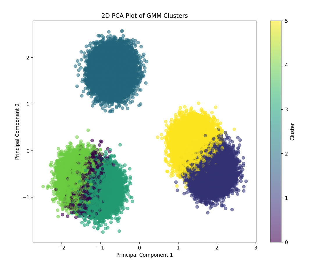
# PCA dimensionality reduction and visualization
pca = PCA(n_components=2)
X_pca = pca.fit_transform(X_scaled)

plt.figure(figsize=(10, 8))
plt.scatter(X_pca[:, 0], X_pca[:, 1], c=labels, cmap='viridis', alpha=0.5)
plt.title('2D PCA Plot of GMM Clusters')
plt.xlabel('Principal Component 1')
plt.ylabel('Principal Component 2')
plt.colorbar(label='Cluster')
plt.show()

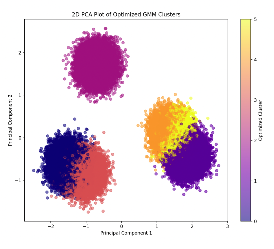
6. Algorithm Optimization

Set iteration count and initialization parameters for the GMM model to improve performance.

# Optimize GMM
optimized_gmm = GaussianMixture(n_components=best_n_components, covariance_type='full', max_iter=500, n_init=10, random_state=42)
optimized_gmm.fit(X_scaled)
optimized_labels = optimized_gmm.predict(X_scaled)

# Update DataFrame
df['OptimizedCluster'] = optimized_labels

# Visualize optimized results
fig = plt.figure(figsize=(10, 8))
ax = fig.add_subplot(111, projection='3d')
scatter = ax.scatter(df['Feature1'], df['Feature2'], df['Feature3'], c=optimized_labels, cmap='plasma', alpha=0.5)
legend1 = ax.legend(*scatter.legend_elements(), title="Optimized Clusters")
ax.add_artist(legend1)
ax.set_title('3D Scatter Plot of Optimized GMM Clusters')
ax.set_xlabel('Feature1')
ax.set_ylabel('Feature2')
ax.set_zlabel('Feature3')
plt.show()

# PCA dimensionality reduction and visualization
X_pca_optimized = pca.fit_transform(X_scaled)

plt.figure(figsize=(10, 8))
plt.scatter(X_pca_optimized[:, 0], X_pca_optimized[:, 1], c=optimized_labels, cmap='plasma', alpha=0.5)
plt.title('2D PCA Plot of Optimized GMM Clusters')
plt.xlabel('Principal Component 1')
plt.ylabel('Principal Component 2')
plt.colorbar(label='Optimized Cluster')
plt.show()

7. Evaluate the Model

Evaluate the effectiveness of GMM clustering, such as calculating the silhouette score.

from sklearn.metrics import silhouette_score

# Calculate silhouette score
silhouette_avg = silhouette_score(X_scaled, optimized_labels)
print(f'Silhouette Score: {silhouette_avg:.3f}')

This case study demonstrates the process of clustering large-scale data using GMM, including data standardization, determining the optimal number of components, applying GMM, and visualizing results through complex visualizations. Additionally, by adjusting the iterations and initialization of GMM, the performance of the model is enhanced.

Alright, that’s all for today’s sharing!

If you like this kind of article, remember to like and bookmark it~