Comprehensive Collection of Common PyTorch Code Snippets

The best resource for PyTorch is the official documentation. This article is a collection of common PyTorch code snippets, with some modifications based on reference material [1] (Zhang Hao: PyTorch Cookbook) for easier lookup during use.

Basic Configuration

Import Packages and Check Versions

import torch
import torch.nn as nn
import torchvision
print(torch.__version__)
print(torch.version.cuda)
print(torch.backends.cudnn.version())
print(torch.cuda.get_device_name(0))

Reproducibility

Complete reproducibility cannot be guaranteed across different hardware devices (CPU, GPU), even with the same random seed. However, reproducibility should be ensured on the same device. The specific approach is to fix the random seed for torch at the start of the program and also fix the random seed for numpy.

np.random.seed(0)
torch.manual_seed(0)
torch.cuda.manual_seed_all(0)

torch.backends.cudnn.deterministic = True
torch.backends.cudnn.benchmark = False

GPU Configuration

If only one GPU is needed

# Device configuration
device = torch.device('cuda' if torch.cuda.is_available() else 'cpu')

If multiple GPUs are needed, such as GPU 0 and 1.

import os
os.environ['CUDA_VISIBLE_DEVICES'] = '0,1'

You can also set the GPU when running code from the command line:

CUDA_VISIBLE_DEVICES=0,1 python train.py

Clear GPU memory

torch.cuda.empty_cache()

You can also use the command line to reset the GPU:

nvidia-smi --gpu-reset -i [gpu_id]

Tensor Processing

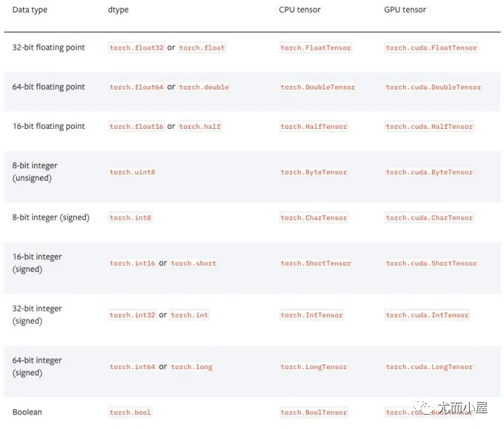
Tensor Data Types

PyTorch has 9 types of CPU tensors and 9 types of GPU tensors.

Basic Tensor Information

tensor = torch.randn(3,4,5)
print(tensor.type())  # Data type
print(tensor.size())  # Tensor shape, a tuple
print(tensor.dim())   # Number of dimensions

Named Tensors

Naming tensors is a very useful method, allowing convenient indexing or other operations using dimension names, greatly improving readability and usability, and preventing errors.

# Before PyTorch 1.3, comments were needed
# Tensor[N, C, H, W]
images = torch.randn(32, 3, 56, 56)
images.sum(dim=1)
images.select(dim=1, index=0)

# After PyTorch 1.3
NCHW = ['N', 'C', 'H', 'W']
images = torch.randn(32, 3, 56, 56, names=NCHW)
images.sum('C')
images.select('C', index=0)
# You can also set it this way
tensor = torch.rand(3,4,1,2,names=('C', 'N', 'H', 'W'))
# Use align_to to conveniently sort dimensions
tensor = tensor.align_to('N', 'C', 'H', 'W')

Data Type Conversion

# Set default type, FloatTensor is much faster than DoubleTensor in PyTorch
torch.set_default_tensor_type(torch.FloatTensor)

# Type conversion
tensor = tensor.cuda()
tensor = tensor.cpu()
tensor = tensor.float()
tensor = tensor.long()

torch.Tensor and np.ndarray Conversion

All CPU tensors except CharTensor support conversion to numpy format and back.

ndarray = tensor.cpu().numpy()
tensor = torch.from_numpy(ndarray).float()
tensor = torch.from_numpy(ndarray.copy()).float() # If ndarray has negative stride.

Torch.tensor and PIL.Image Conversion

# Tensors in PyTorch are in [N, C, H, W] order by default, and the data range is [0,1], needs transposing and normalization
# torch.Tensor -> PIL.Image
image = PIL.Image.fromarray(torch.clamp(tensor*255, min=0, max=255).byte().permute(1,2,0).cpu().numpy())
image = torchvision.transforms.functional.to_pil_image(tensor)  # Equivalently way

# PIL.Image -> torch.Tensor
path = r'./figure.jpg'
tensor = torch.from_numpy(np.asarray(PIL.Image.open(path))).permute(2,0,1).float() / 255
tensor = torchvision.transforms.functional.to_tensor(PIL.Image.open(path)) # Equivalently way

np.ndarray and PIL.Image Conversion

image = PIL.Image.fromarray(ndarray.astype(np.uint8))
darray = np.asarray(PIL.Image.open(path))

Extracting Value from a Tensor Containing One Element

value = torch.rand(1).item()

Tensor Reshaping

# Usually requires reshaping when inputting tensors from convolution layers to fully connected layers,
# Compared to torch.view, torch.reshape can automatically handle cases where the input tensor is not contiguous

tensor = torch.rand(2,3,4)
shape = (6, 4)
tensor = torch.reshape(tensor, shape)

Shuffle Order

tensor = tensor[torch.randperm(tensor.size(0))]  # Shuffle the first dimension

Horizontal Flip

# PyTorch does not support negative step operations like tensor[::-1], horizontal flipping can be achieved through tensor indexing
# Assuming the tensor dimension is [N, D, H, W].

tensor = tensor[:,:,:,torch.arange(tensor.size(3) - 1, -1, -1).long()]

Copying Tensors

# Operation                 |  New/Shared memory | Still in computation graph |
tensor.clone()            # |        New         |          Yes               |
tensor.detach()           # |      Shared        |          No                |
tensor.detach.clone()()   # |        New         |          No                |

Tensor Concatenation

''' 
Note the difference between torch.cat and torch.stack: torch.cat concatenates along the specified dimension,
while torch.stack adds a new dimension. For example, when the parameters are 3 tensors of size 10x5, the result of torch.cat is a tensor of size 30x5,
while the result of torch.stack is a tensor of size 3x10x5.
'''
tensor = torch.cat(list_of_tensors, dim=0)
tensor = torch.stack(list_of_tensors, dim=0)

Convert Integer Labels to One-Hot Encoding

# PyTorch's labels start from 0 by default
tensor = torch.tensor([0, 2, 1, 3])
N = tensor.size(0)
num_classes = 4
one_hot = torch.zeros(N, num_classes).long()
one_hot.scatter_(dim=1, index=torch.unsqueeze(tensor, dim=1), src=torch.ones(N, num_classes).long())

Get Non-Zero Elements

torch.nonzero(tensor)               # index of non-zero elements
torch.nonzero(tensor==0)            # index of zero elements
torch.nonzero(tensor).size(0)       # number of non-zero elements
torch.nonzero(tensor == 0).size(0)  # number of zero elements

Check if Two Tensors are Equal

torch.allclose(tensor1, tensor2)  # float tensor
torch.equal(tensor1, tensor2)     # int tensor

Tensor Expansion

# Expand tensor of shape 64*512 to shape 64*512*7*7.
tensor = torch.rand(64,512)
torch.reshape(tensor, (64, 512, 1, 1)).expand(64, 512, 7, 7)

Matrix Multiplication

# Matrix multiplication: (m*n) * (n*p) -> (m*p).
result = torch.mm(tensor1, tensor2)

# Batch matrix multiplication: (b*m*n) * (b*n*p) -> (b*m*p)
result = torch.bmm(tensor1, tensor2)

# Element-wise multiplication.
result = tensor1 * tensor2

Calculate Pairwise Euclidean Distances Between Two Sets of Data

Utilizing broadcasting mechanism

dist = torch.sqrt(torch.sum((X1[:,None,:] - X2) ** 2, dim=2))

Model Definition and Operations

An Example of a Simple Two-Layer Convolutional Network

# convolutional neural network (2 convolutional layers)
class ConvNet(nn.Module):
    def __init__(self, num_classes=10):
        super(ConvNet, self).__init__()
        self.layer1 = nn.Sequential(
            nn.Conv2d(1, 16, kernel_size=5, stride=1, padding=2),
            nn.BatchNorm2d(16),
            nn.ReLU(),
            nn.MaxPool2d(kernel_size=2, stride=2))
        self.layer2 = nn.Sequential(
            nn.Conv2d(16, 32, kernel_size=5, stride=1, padding=2),
            nn.BatchNorm2d(32),
            nn.ReLU(),
            nn.MaxPool2d(kernel_size=2, stride=2))
        self.fc = nn.Linear(7*7*32, num_classes)

    def forward(self, x):
        out = self.layer1(x)
        out = self.layer2(out)
        out = out.reshape(out.size(0), -1)
        out = self.fc(out)
        return out

model = ConvNet(num_classes).to(device)

The computation and visualization of convolution layers can be aided by this website.

Bilinear Pooling

X = torch.reshape(N, D, H * W)                        # Assume X has shape N*D*H*W
X = torch.bmm(X, torch.transpose(X, 1, 2)) / (H * W)  # Bilinear pooling
assert X.size() == (N, D, D)
X = torch.reshape(X, (N, D * D))
X = torch.sign(X) * torch.sqrt(torch.abs(X) + 1e-5)   # Signed-sqrt normalization
X = torch.nn.functional.normalize(X)                  # L2 normalization

Multi-GPU Synchronized Batch Normalization

When using torch.nn.DataParallel to run code on multiple GPUs, PyTorch’s default operation for BN layers is to compute the mean and variance independently on each card. Synchronized BN uses data from all cards to compute the mean and variance of the BN layer, alleviating the issue of inaccurate mean and variance estimates when the batch size is small, making it an effective performance enhancement technique in tasks such as object detection.

sync_bn = torch.nn.SyncBatchNorm(num_features, 
                                 eps=1e-05, 
                                 momentum=0.1, 
                                 affine=True, 
                                 track_running_stats=True)

Convert All BN Layers of an Existing Network to Synchronized BN Layers

def convertBNtoSyncBN(module, process_group=None):
    '''Recursively replace all BN layers to SyncBN layer.

    Args:
        module[torch.nn.Module]. Network
    '''
    if isinstance(module, torch.nn.modules.batchnorm._BatchNorm):
        sync_bn = torch.nn.SyncBatchNorm(module.num_features, module.eps, module.momentum, 
                                         module.affine, module.track_running_stats, process_group)
        sync_bn.running_mean = module.running_mean
        sync_bn.running_var = module.running_var
        if module.affine:
            sync_bn.weight = module.weight.clone().detach()
            sync_bn.bias = module.bias.clone().detach()
        return sync_bn
    else:
        for name, child_module in module.named_children():
            setattr(module, name, convert_syncbn_model(child_module, process_group=process_group))
        return module

Similar to BN Moving Average

To implement an operation similar to BN moving average, in the forward function, use in-place operations to assign values to the moving average.

class BN(torch.nn.Module)
    def __init__(self):
        ...
        self.register_buffer('running_mean', torch.zeros(num_features))

    def forward(self, X):
        ...
        self.running_mean += momentum * (current - self.running_mean)

Calculate Total Number of Parameters in the Model

num_parameters = sum(torch.numel(parameter) for parameter in model.parameters())

View Parameters in the Network

You can view all the trainable parameters (including those inherited from parent classes) through model.state_dict() or model.named_parameters().

params = list(model.named_parameters())
(name, param) = params[28]
print(name)
print(param.grad)
print('-------------------------------------------------')
(name2, param2) = params[29]
print(name2)
print(param2.grad)
print('----------------------------------------------------')
(name1, param1) = params[30]
print(name1)
print(param1.grad)

Model Visualization (Using pytorchviz)

szagoruyko/pytorchvizgithub.com

Similar to Keras’s model.summary(), use pytorch-summary to output model information.

sksq96/pytorch-summarygithub.com

Model Weight Initialization

Note the difference between model.modules() and model.children(): model.modules() iterates through all sub-layers of the model, while model.children() only traverses the first layer of the model.

# Common practice for initialization.
for layer in model.modules():
    if isinstance(layer, torch.nn.Conv2d):
        torch.nn.init.kaiming_normal_(layer.weight, mode='fan_out',
                                      nonlinearity='relu')
        if layer.bias is not None:
            torch.nn.init.constant_(layer.bias, val=0.0)
    elif isinstance(layer, torch.nn.BatchNorm2d):
        torch.nn.init.constant_(layer.weight, val=1.0)
        torch.nn.init.constant_(layer.bias, val=0.0)
    elif isinstance(layer, torch.nn.Linear):
        torch.nn.init.xavier_normal_(layer.weight)
        if layer.bias is not None:
            torch.nn.init.constant_(layer.bias, val=0.0)

# Initialization with given tensor.
layer.weight = torch.nn.Parameter(tensor)

Extract a Specific Layer from the Model

modules() returns an iterator of all modules in the model, allowing access to the innermost layers, such as self.layer1.conv1. There are also corresponding attributes named_children() and named_modules(), which return not only the iterator of modules but also the names of the network layers.

# Extract the first two layers from the model
new_model = nn.Sequential(*list(model.children())[:2]) 
# If you want to extract all convolution layers from the model, you can do it like this:
for layer in model.named_modules():
    if isinstance(layer[1],nn.Conv2d):
         conv_model.add_module(layer[0],layer[1])

Use Pre-trained Models for Some Layers

Note that if the saved model is torch.nn.DataParallel, the current model also needs to be.

model.load_state_dict(torch.load('model.pth'), strict=False)

Load a Model Saved on GPU to CPU

model.load_state_dict(torch.load('model.pth', map_location='cpu'))

Import Corresponding Parts of Another Model into a New Model

When importing parameters from a model, if the structures of the two models are inconsistent, directly importing the parameters will raise an error. The following method can be used to import the same parts from another model into the new model.

# model_new represents the new model
# model_saved represents another model, such as a saved model imported with torch.load
model_new_dict = model_new.state_dict()
model_common_dict = {k:v for k, v in model_saved.items() if k in model_new_dict.keys()}
model_new_dict.update(model_common_dict)
model_new.load_state_dict(model_new_dict)

Data Processing

Calculate Mean and Standard Deviation of the Dataset

import os
import cv2
import numpy as np
from torch.utils.data import Dataset
from PIL import Image

def compute_mean_and_std(dataset):
    # Input PyTorch dataset, output mean and standard deviation
    mean_r = 0
    mean_g = 0
    mean_b = 0

    for img, _ in dataset:
        img = np.asarray(img) # change PIL Image to numpy array
        mean_b += np.mean(img[:, :, 0])
        mean_g += np.mean(img[:, :, 1])
        mean_r += np.mean(img[:, :, 2])

    mean_b /= len(dataset)
    mean_g /= len(dataset)
    mean_r /= len(dataset)

    diff_r = 0
    diff_g = 0
    diff_b = 0

    N = 0

    for img, _ in dataset:
        img = np.asarray(img)

        diff_b += np.sum(np.power(img[:, :, 0] - mean_b, 2))
        diff_g += np.sum(np.power(img[:, :, 1] - mean_g, 2))
        diff_r += np.sum(np.power(img[:, :, 2] - mean_r, 2))

        N += np.prod(img[:, :, 0].shape)

    std_b = np.sqrt(diff_b / N)
    std_g = np.sqrt(diff_g / N)
    std_r = np.sqrt(diff_r / N)

    mean = (mean_b.item() / 255.0, mean_g.item() / 255.0, mean_r.item() / 255.0)
    std = (std_b.item() / 255.0, std_g.item() / 255.0, std_r.item() / 255.0)
    return mean, std

Get Basic Information of Video Data

import cv2
video = cv2.VideoCapture(mp4_path)
height = int(video.get(cv2.CAP_PROP_FRAME_HEIGHT))
width = int(video.get(cv2.CAP_PROP_FRAME_WIDTH))
num_frames = int(video.get(cv2.CAP_PROP_FRAME_COUNT))
fps = int(video.get(cv2.CAP_PROP_FPS))
video.release()

Sample One Frame of Video for Each Segment in TSN

K = self._num_segments
if is_train:
    if num_frames > K:
        # Random index for each segment.
        frame_indices = torch.randint(
            high=num_frames // K, size=(K,), dtype=torch.long)
        frame_indices += num_frames // K * torch.arange(K)
    else:
        frame_indices = torch.randint(
            high=num_frames, size=(K - num_frames,), dtype=torch.long)
        frame_indices = torch.sort(torch.cat((
            torch.arange(num_frames), frame_indices)))[0]
else:
    if num_frames > K:
        # Middle index for each segment.
        frame_indices = num_frames / K // 2
        frame_indices += num_frames // K * torch.arange(K)
    else:
        frame_indices = torch.sort(torch.cat((                               
            torch.arange(num_frames), torch.arange(K - num_frames))))[0]
assert frame_indices.size() == (K,)
return [frame_indices[i] for i in range(K)]

Common Training and Validation Data Preprocessing

The ToTensor operation converts a PIL.Image or an np.ndarray of shape H×W×D, with a value range of [0, 255], to a torch.Tensor of shape D×H×W, with a value range of [0.0, 1.0].

train_transform = torchvision.transforms.Compose([
    torchvision.transforms.RandomResizedCrop(size=224,
                                             scale=(0.08, 1.0)),
    torchvision.transforms.RandomHorizontalFlip(),
    torchvision.transforms.ToTensor(),
    torchvision.transforms.Normalize(mean=(0.485, 0.456, 0.406),
                                     std=(0.229, 0.224, 0.225)),
 ])
 val_transform = torchvision.transforms.Compose([
    torchvision.transforms.Resize(256),
    torchvision.transforms.CenterCrop(224),
    torchvision.transforms.ToTensor(),
    torchvision.transforms.Normalize(mean=(0.485, 0.456, 0.406),
                                     std=(0.229, 0.224, 0.225)),
])

Model Training and Testing

Classification Model Training Code

# Loss and optimizer
criterion = nn.CrossEntropyLoss()
optimizer = torch.optim.Adam(model.parameters(), lr=learning_rate)

# Train the model
total_step = len(train_loader)
for epoch in range(num_epochs):
    for i ,(images, labels) in enumerate(train_loader):
        images = images.to(device)
        labels = labels.to(device)

        # Forward pass
        outputs = model(images)
        loss = criterion(outputs, labels)

        # Backward and optimizer
        optimizer.zero_grad()
        loss.backward()
        optimizer.step()

        if (i+1) % 100 == 0:
            print('Epoch: [{}/{}], Step: [{}/{}], Loss: {}'
                  .format(epoch+1, num_epochs, i+1, total_step, loss.item()))

Classification Model Testing Code

# Test the model
model.eval()  # eval mode(batch norm uses moving mean/variance 
              #instead of mini-batch mean/variance)
with torch.no_grad():
    correct = 0
    total = 0
    for images, labels in test_loader:
        images = images.to(device)
        labels = labels.to(device)
        outputs = model(images)
        _, predicted = torch.max(outputs.data, 1)
        total += labels.size(0)
        correct += (predicted == labels).sum().item()

    print('Test accuracy of the model on the 10000 test images: {} %'
          .format(100 * correct / total))

Custom Loss

Inherit from the torch.nn.Module class to write your own loss.

class MyLoss(torch.nn.Module):
    def __init__(self):
        super(MyLoss, self).__init__()

    def forward(self, x, y):
        loss = torch.mean((x - y) ** 2)
        return loss

Label Smoothing

Create a label_smoothing.py file and reference it in the training code, replacing cross-entropy loss with LSR. The content of label_smoothing.py is as follows:

import torch
import torch.nn as nn


class LSR(nn.Module):

    def __init__(self, e=0.1, reduction='mean'):
        super().__init__()

        self.log_softmax = nn.LogSoftmax(dim=1)
        self.e = e
        self.reduction = reduction

    def _one_hot(self, labels, classes, value=1):
        """
            Convert labels to one hot vectors

        Args:
            labels: torch tensor in format [label1, label2, label3, ...]
            classes: int, number of classes
            value: label value in one hot vector, default to 1

        Returns:
            return one hot format labels in shape [batchsize, classes]
        """

        one_hot = torch.zeros(labels.size(0), classes)

        #labels and value_added  size must match
        labels = labels.view(labels.size(0), -1)
        value_added = torch.Tensor(labels.size(0), 1).fill_(value)

        value_added = value_added.to(labels.device)
        one_hot = one_hot.to(labels.device)

        one_hot.scatter_add_(1, labels, value_added)

        return one_hot

    def _smooth_label(self, target, length, smooth_factor):
        """convert targets to one-hot format, and smooth
        them.
        Args:
            target: target in form with [label1, label2, label_batchsize]
            length: length of one-hot format(number of classes)
            smooth_factor: smooth factor for label smooth

        Returns:
            smoothed labels in one hot format
        """
        one_hot = self._one_hot(target, length, value=1 - smooth_factor)
        one_hot += smooth_factor / (length - 1)

        return one_hot.to(target.device)

    def forward(self, x, target):

        if x.size(0) != target.size(0):
            raise ValueError('Expected input batchsize ({}) to match target batch_size({})'
                    .format(x.size(0), target.size(0)))

        if x.dim() < 2:
            raise ValueError('Expected input tensor to have least 2 dimensions(got {})'
                    .format(x.size(0)))

        if x.dim() != 2:
            raise ValueError('Only 2 dimension tensor are implemented, (got {})'
                    .format(x.size()))


        smoothed_target = self._smooth_label(target, x.size(1), self.e)
        x = self.log_softmax(x)
        loss = torch.sum(- x * smoothed_target, dim=1)

        if self.reduction == 'none':
            return loss

        elif self.reduction == 'sum':
            return torch.sum(loss)

        elif self.reduction == 'mean':
            return torch.mean(loss)

        else:
            raise ValueError('unrecognized option, expect reduction to be one of none, mean, sum')

Alternatively, you can implement label smoothing directly in the training file.

for images, labels in train_loader:
    images, labels = images.cuda(), labels.cuda()
    N = labels.size(0)
    # C is the number of classes.
    smoothed_labels = torch.full(size=(N, C), fill_value=0.1 / (C - 1)).cuda()
    smoothed_labels.scatter_(dim=1, index=torch.unsqueeze(labels, dim=1), value=0.9)

    score = model(images)
    log_prob = torch.nn.functional.log_softmax(score, dim=1)
    loss = -torch.sum(log_prob * smoothed_labels) / N
    optimizer.zero_grad()
    loss.backward()
    optimizer.step()

Mixup Training

beta_distribution = torch.distributions.beta.Beta(alpha, alpha)
for images, labels in train_loader:
    images, labels = images.cuda(), labels.cuda()

    # Mixup images and labels.
    lambda_ = beta_distribution.sample([]).item()
    index = torch.randperm(images.size(0)).cuda()
    mixed_images = lambda_ * images + (1 - lambda_) * images[index, :]
    label_a, label_b = labels, labels[index]

    # Mixup loss.
    scores = model(mixed_images)
    loss = (lambda_ * loss_function(scores, label_a)
            + (1 - lambda_) * loss_function(scores, label_b))
    optimizer.zero_grad()
    loss.backward()
    optimizer.step()

L1 Regularization

l1_regularization = torch.nn.L1Loss(reduction='sum')
loss = ...  # Standard cross-entropy loss

for param in model.parameters():
    loss += torch.sum(torch.abs(param))
loss.backward()

Do Not Apply Weight Decay to Bias Terms

Weight decay in PyTorch is equivalent to L2 regularization.

bias_list = (param for name, param in model.named_parameters() if name[-4:] == 'bias')
others_list = (param for name, param in model.named_parameters() if name[-4:] != 'bias')
parameters = [{'parameters': bias_list, 'weight_decay': 0},                
              {'parameters': others_list}]
optimizer = torch.optim.SGD(parameters, lr=1e-2, momentum=0.9, weight_decay=1e-4)

Gradient Clipping

torch.nn.utils.clip_grad_norm_(model.parameters(), max_norm=20)

Get Current Learning Rate

# If there is one global learning rate (which is the common case).
lr = next(iter(optimizer.param_groups))['lr']

# If there are multiple learning rates for different layers.
all_lr = []
for param_group in optimizer.param_groups:
    all_lr.append(param_group['lr'])

Another method is to check the current lr in the training code of a batch: optimizer.param_groups[0]['lr'].

Learning Rate Decay

# Reduce learning rate when validation accuracy plateaus.
scheduler = torch.optim.lr_scheduler.ReduceLROnPlateau(optimizer, mode='max', patience=5, verbose=True)
for t in range(0, 80):
    train(...)
    val(...)
    scheduler.step(val_acc)

# Cosine annealing learning rate.
scheduler = torch.optim.lr_scheduler.CosineAnnealingLR(optimizer, T_max=80)
# Reduce learning rate by 10 at given epochs.
scheduler = torch.optim.lr_scheduler.MultiStepLR(optimizer, milestones=[50, 70], gamma=0.1)
for t in range(0, 80):
    scheduler.step()    
    train(...)
    val(...)

# Learning rate warmup by 10 epochs.
scheduler = torch.optim.lr_scheduler.LambdaLR(optimizer, lr_lambda=lambda t: t / 10)
for t in range(0, 10):
    scheduler.step()
    train(...)
    val(...)

Optimizer Chaining Update

Starting from version 1.4, torch.optim.lr_scheduler supports chaining, allowing users to define two schedulers and alternate their use during training.

import torch
from torch.optim import SGD
from torch.optim.lr_scheduler import ExponentialLR, StepLR
model = [torch.nn.Parameter(torch.randn(2, 2, requires_grad=True))]
optimizer = SGD(model, 0.1)
scheduler1 = ExponentialLR(optimizer, gamma=0.9)
scheduler2 = StepLR(optimizer, step_size=3, gamma=0.1)
for epoch in range(4):
    print(epoch, scheduler2.get_last_lr()[0])
    optimizer.step()
    scheduler1.step()
    scheduler2.step()

Model Training Visualization

PyTorch can use TensorBoard to visualize the training process. Install and run TensorBoard.

pip install tensorboard
tensorboard --logdir=runs

Use the SummaryWriter class to collect and visualize the corresponding data. To facilitate viewing, different folders can be used, such as ‘Loss/train’ and ‘Loss/test’.

from torch.utils.tensorboard import SummaryWriter
import numpy as np

writer = SummaryWriter()

for n_iter in range(100):
    writer.add_scalar('Loss/train', np.random.random(), n_iter)
    writer.add_scalar('Loss/test', np.random.random(), n_iter)
    writer.add_scalar('Accuracy/train', np.random.random(), n_iter)
    writer.add_scalar('Accuracy/test', np.random.random(), n_iter)

Save and Load Checkpoints

To be able to resume training, we need to save both the model and optimizer states, as well as the current training epoch.

start_epoch = 0
# Load checkpoint.
if resume: # resume is a parameter, set to 0 for first training, 1 for resuming training
    model_path = os.path.join('model', 'best_checkpoint.pth.tar')
    assert os.path.isfile(model_path)
    checkpoint = torch.load(model_path)
    best_acc = checkpoint['best_acc']
    start_epoch = checkpoint['epoch']
    model.load_state_dict(checkpoint['model'])
    optimizer.load_state_dict(checkpoint['optimizer'])
    print('Load checkpoint at epoch {}.'.format(start_epoch))
    print('Best accuracy so far {}.'.format(best_acc))

# Train the model
for epoch in range(start_epoch, num_epochs): 
    ... 

    # Test the model
    ...

    # save checkpoint
    is_best = current_acc > best_acc
    best_acc = max(current_acc, best_acc)
    checkpoint = {
        'best_acc': best_acc,
        'epoch': epoch + 1,
        'model': model.state_dict(),
        'optimizer': optimizer.state_dict(),
    }
    model_path = os.path.join('model', 'checkpoint.pth.tar')
    best_model_path = os.path.join('model', 'best_checkpoint.pth.tar')
    torch.save(checkpoint, model_path)
    if is_best:
        shutil.copy(model_path, best_model_path)

Extract Convolution Features from Pre-trained ImageNet Model

# VGG-16 relu5-3 feature.
model = torchvision.models.vgg16(pretrained=True).features[:-1]
# VGG-16 pool5 feature.
model = torchvision.models.vgg16(pretrained=True).features
# VGG-16 fc7 feature.
model = torchvision.models.vgg16(pretrained=True)
model.classifier = torch.nn.Sequential(*list(model.classifier.children())[:-3])
# ResNet GAP feature.
model = torchvision.models.resnet18(pretrained=True)
model = torch.nn.Sequential(collections.OrderedDict(
    list(model.named_children())[:-1]))

with torch.no_grad():
    model.eval()
    conv_representation = model(image)

Extract Multiple Convolution Features from Pre-trained ImageNet Model

class FeatureExtractor(torch.nn.Module):
    """Helper class to extract several convolution features from the given
    pre-trained model.

    Attributes:
        _model, torch.nn.Module.
        _layers_to_extract, list<str> or set<str>

    Example:
        >>> model = torchvision.models.resnet152(pretrained=True)
        >>> model = torch.nn.Sequential(collections.OrderedDict(
                list(model.named_children())[:-1]))
        >>> conv_representation = FeatureExtractor(
                pretrained_model=model,
                layers_to_extract={'layer1', 'layer2', 'layer3', 'layer4'})(image)
    """
    def __init__(self, pretrained_model, layers_to_extract):
        torch.nn.Module.__init__(self)
        self._model = pretrained_model
        self._model.eval()
        self._layers_to_extract = set(layers_to_extract)

    def forward(self, x):
        with torch.no_grad():
            conv_representation = []
            for name, layer in self._model.named_children():
                x = layer(x)
                if name in self._layers_to_extract:
                    conv_representation.append(x)
            return conv_representation

Fine-tune Fully Connected Layer

model = torchvision.models.resnet18(pretrained=True)
for param in model.parameters():
    param.requires_grad = False
model.fc = nn.Linear(512, 100)  # Replace the last fc layer
optimizer = torch.optim.SGD(model.fc.parameters(), lr=1e-2, momentum=0.9, weight_decay=1e-4)

Fine-tune Fully Connected Layer with Higher Learning Rate, Convolution Layers with Lower Learning Rate

model = torchvision.models.resnet18(pretrained=True)
finetuned_parameters = list(map(id, model.fc.parameters()))
conv_parameters = (p for p in model.parameters() if id(p) not in finetuned_parameters)
parameters = [{'params': conv_parameters, 'lr': 1e-3}, 
              {'params': model.fc.parameters()}]
optimizer = torch.optim.SGD(parameters, lr=1e-2, momentum=0.9, weight_decay=1e-4)

Other Considerations

• Do not use overly large linear layers. Because nn.Linear(m,n) uses a lot of memory, large linear layers can easily exceed the existing GPU memory.
• Do not use RNNs on overly long sequences. Because RNN backpropagation uses the BPTT algorithm, the memory required is linearly related to the length of the input sequence.
• Switch the network state with model.train() and model.eval() before model(x).
• Code blocks that do not require gradient calculation should be enclosed in with torch.no_grad().
• The difference between model.eval() and torch.no_grad() is that model.eval() switches the network to test mode, for example, BN and dropout use different calculation methods in training and testing phases. torch.no_grad() disables PyTorch’s automatic differentiation mechanism for tensors, reducing memory usage and speeding up computation; the results cannot be used for loss.backward().
• model.zero_grad() will zero out the gradients of all parameters in the model, while optimizer.zero_grad() will only zero out the gradients of the parameters passed to it.
• torch.nn.CrossEntropyLoss does not require the input to go through Softmax. torch.nn.CrossEntropyLoss is equivalent to torch.nn.functional.log_softmax + torch.nn.NLLLoss.
• Use optimizer.zero_grad() to clear accumulated gradients before loss.backward().
• In torch.utils.data.DataLoader, try to set pin_memory=True; for particularly small datasets like MNIST, setting pin_memory=False can be faster. The setting for num_workers needs to be found through experimentation for the fastest value.
• Use del to delete unnecessary intermediate variables in a timely manner to save GPU memory. Using in-place operations can also save GPU memory, such as:

x = torch.nn.functional.relu(x, inplace=True)

Reduce data transfer between CPU and GPU. For example, if you want to know the loss and accuracy of each mini-batch in an epoch, accumulating them on the GPU and transferring them back to the CPU at the end of the epoch is faster than transferring them back after each mini-batch. Using half-precision floating-point numbers half() can provide some speed improvement, with specific efficiency depending on the GPU model. Care should be taken to avoid stability issues caused by low numerical precision. Regularly use assert tensor.size() == (N, D, H, W) as a debugging tool to ensure tensor dimensions are as expected. Avoid using one-dimensional tensors except for labeling y; use n*1 two-dimensional tensors instead to avoid unexpected results in one-dimensional tensor calculations. Time the execution of different parts of the code:

with torch.autograd.profiler.profile(enabled=True, use_cuda=False) as profile:    
  ...print(profile)# Or run python -m torch.utils.bottleneck main.py in the command line

Use TorchSnooper to debug PyTorch code; the program will automatically print the shape, data type, device, and gradient requirement of each tensor executed during the execution.

# pip install torchsnooper
import torchsnooper# Use the decorator @torchsnooper.snoop() for functions

# If not a function, use the with statement to activate TorchSnooper, putting the training loop inside the with statement.
with torchsnooper.snoop():    
  Original code

https://github.com/zasdfgbnm/TorchSnooper github.com Model interpretability, use the captum library: https://captum.ai/captum.ai

References

• Zhang Hao: PyTorch Cookbook, https://zhuanlan.zhihu.com/p/59205847?
• PyTorch Official Documentation and Examples
• https://pytorch.org/docs/stable/notes/faq.html
• https://github.com/szagoruyko/pytorchviz
• https://github.com/sksq96/pytorch-summary, etc.

Academic sharing, Source丨https://zhuanlan.zhihu.com/p/104019160