Machine Learning
Author: louwill
Machine Learning Lab
Although deep learning is currently dominant, Boosting algorithms represented by XGBoost, LightGBM, and CatBoost still have a wide range of applications. Excluding the unstructured data applications suitable for deep learning, such as images, text, speech, and video, Boosting algorithms remain the first choice for structured data with fewer training samples. This article first briefly explains the connections and differences among the three major Boosting algorithms mentioned above, followed by a comparison of the three algorithms using a practical data case. Then, it introduces common hyperparameter tuning methods for Boosting algorithms, including random search, grid search, and Bayesian optimization, along with corresponding code examples.
Comparison of Three Major Boosting Algorithms
First, XGBoost, LightGBM, and CatBoost are currently classic state-of-the-art (SOTA) Boosting algorithms, all classified under the gradient boosting decision tree algorithm series. All three models are ensemble learning frameworks supported by decision trees, where XGBoost is an improvement over the original version of the GBDT algorithm, while LightGBM and CatBoost are further optimized based on XGBoost, each with its own advantages in terms of accuracy and speed.
The details of the principles of the three models are not discussed in this article; please refer to the document “Machine Learning Formula Derivation and Code Implementation 30 Lectures.pdf” for more information. So, what are the major differences among these three Boosting algorithms? There are mainly two aspects. The first is that the construction methods of the trees in the three models differ. XGBoost uses a level-wise growth strategy for decision trees, LightGBM uses a leaf-wise growth strategy, while CatBoost employs a symmetric tree structure, where its decision trees are all complete binary trees. The second significant difference lies in the handling of categorical features. XGBoost does not have the capability to automatically handle categorical features; we need to manually transform them into numerical values before inputting them into the model. In LightGBM, categorical feature names need to be specified, and the algorithm can handle them automatically. CatBoost is known for its ability to handle categorical features efficiently through techniques such as target variable statistics.
Next, we will use the Kaggle 2015 Flight Delay Dataset as an example to experiment with the XGBoost, LightGBM, and CatBoost models. Figure 1 provides an overview of the flights dataset.

Figure 2 Flights Dataset
The complete dataset contains over 5 million flight records with 31 features. For demonstration purposes, we will sample 1% of the original dataset and select 11 features. After preprocessing, we will reconstruct the training dataset with the goal of building a binary classification model to predict whether flights are delayed. The data reading and simple preprocessing process is shown in Code 1.
Code 1 Data Processing
# Import pandas and sklearn data splitting module
import pandas as pd
from sklearn.model_selection import train_test_split

# Read the flights dataset
flights = pd.read_csv('flights.csv')

# Sample 1% of the dataset
flights = flights.sample(frac=0.01, random_state=10)

# Feature sampling, selecting 11 specific features
flights = flights["MONTH", "DAY", "DAY_OF_WEEK", "AIRLINE", "FLIGHT_NUMBER", "DESTINATION_AIRPORT", "ORIGIN_AIRPORT", "AIR_TIME", "DEPARTURE_TIME", "DISTANCE", "ARRIVAL_DELAY"]

# Discretize labels, only delays over 10 minutes are considered delays
flights["ARRIVAL_DELAY"] = (flights["ARRIVAL_DELAY"] > 10) * 1

# Categorical features
cat_cols = ["AIRLINE", "FLIGHT_NUMBER", "DESTINATION_AIRPORT", "ORIGIN_AIRPORT"]

# Encode categorical features
for item in cat_cols:
    flights[item] = flights[item].astype("category").cat.codes + 1

# Split the dataset
X_train, X_test, y_train, y_test = train_test_split(
    flights.drop(["ARRIVAL_DELAY"], axis=1),
    flights["ARRIVAL_DELAY"],
    random_state=10, test_size=0.3)

# Print the sizes of the split datasets
print(X_train.shape, y_train.shape, X_test.shape, y_test.shape)
Output:
(39956, 10) (39956,) (17125, 10) (17125,)In Code 1, we first read the original flights dataset. Since the original dataset is too large, we sample 1% and select 11 features to create a dataset with 57081 records and 11 features. We then perform simple preprocessing on the sampled dataset, first discretizing the training labels, converting delays greater than 10 minutes to 1 (delayed) and delays less than 10 minutes to 0 (not delayed). Next, we encode the categorical features such as “Airline,” “Flight Number,” “Destination Airport,” and “Origin Airport.” Finally, we split the dataset, resulting in 39956 training samples and 17125 test samples.
XGBoost
Next, we will test the performance of the three models on this dataset, starting with XGBoost, as shown in Code 2.
Code 2 XGBoost
# Import xgboost module
import xgboost as xgb

# Import model evaluation AUC function
from sklearn.metrics import roc_auc_score

# Set model hyperparameters
params = {
    'booster': 'gbtree',
    'objective': 'binary:logistic',
    'gamma': 0.1,
    'max_depth': 8,
    'lambda': 2,
    'subsample': 0.7,
    'colsample_bytree': 0.7,
    'min_child_weight': 3,
    'eta': 0.001,
    'seed': 1000,
    'nthread': 4,
}

# Wrap xgboost dataset
dtrain = xgb.DMatrix(X_train, y_train)

# Number of training rounds, i.e., number of trees
num_rounds = 500

# Train the model
model_xgb = xgb.train(params, dtrain, num_rounds)

# Predict on the test set
dtest = xgb.DMatrix(X_test)
y_pred = model_xgb.predict(dtest)
print('AUC of test set based on XGBoost: ', roc_auc_score(y_test, y_pred))
Output:
AUC of test set based on XGBoost: 0.6845368959487046In Code 2, we tested the performance of XGBoost on the flights dataset, imported the relevant modules, and set the model hyperparameters. We then fitted the XGBoost model based on the training set, and finally used the trained model to predict the test set, obtaining an AUC of 0.6845 for the test set.
LightGBM
The testing process of LightGBM on the flights dataset is shown in Code 3.
Code 3 LightGBM
# Import lightgbm module
import lightgbm as lgb
dtrain = lgb.Dataset(X_train, label=y_train)
params = {"max_depth": 5, "learning_rate": 0.05, "num_leaves": 500, "n_estimators": 300}

# Specify categorical features
cate_features_name = ["MONTH", "DAY", "DAY_OF_WEEK", "AIRLINE", "DESTINATION_AIRPORT", "ORIGIN_AIRPORT"]

# Fit the lightgbm model
model_lgb = lgb.train(params, dtrain, categorical_feature=cate_features_name)

# Predict on the test set
y_pred = model_lgb.predict(X_test)
print('AUC of test set based on LightGBM: ', roc_auc_score(y_test, y_pred))
Output:
AUC of test set based on LightGBM: 0.6873707383550387In Code 3, we tested the performance of LightGBM on the flights dataset, imported the relevant modules, and set the model hyperparameters. We then fitted the LightGBM model based on the training set, and finally used the trained model to predict the test set, obtaining an AUC of 0.6873, which is similar to XGBoost.
CatBoost
The testing process of CatBoost on the flights dataset is shown in Code 4.
Code 4 CatBoost
# Import catboost module
import catboost as cb

# Categorical feature indices
cat_features_index = [0, 1, 2, 3, 4, 5, 6]

# Create CatBoost model instance
model_cb = cb.CatBoostClassifier(eval_metric="AUC", one_hot_max_size=50, depth=6, iterations=300, l2_leaf_reg=1, learning_rate=0.1)

# Fit the CatBoost model
model_cb.fit(X_train, y_train, cat_features=cat_features_index)

# Predict on the test set
y_pred = model_cb.predict(X_test)
print('AUC of test set based on CatBoost: ', roc_auc_score(y_test, y_pred))
Output:
AUC of test set based on CatBoost: 0.5463773041667715In Code 4, we tested the performance of CatBoost on the flights dataset, imported the relevant modules, and set the model hyperparameters. We then fitted the CatBoost model based on the training set, and finally used the trained model to predict the test set, obtaining an AUC of 0.54, which is significantly lower compared to XGBoost and LightGBM. Table 1 shows the comprehensive comparison results of the three models on the flights dataset.
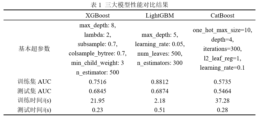
From the comprehensive comparison results in Table 1, LightGBM outperforms both XGBoost and CatBoost in terms of accuracy and speed. Of course, we only compared the three models directly on the dataset without further data feature engineering and hyperparameter tuning; the results in Table 1 can be further optimized.
Common Hyperparameter Tuning Methods
In machine learning models, there are numerous parameters that need to be set manually beforehand, such as the batch size for training neural networks and tree-related parameters for ensemble learning models like XGBoost. We refer to these parameters that are not obtained through model training as hyperparameters. The process of manually adjusting hyperparameters is what we commonly know as tuning. Common tuning methods in machine learning include grid search, random search, and Bayesian optimization.
Grid Search
Grid search is a commonly used hyperparameter tuning method, often used to optimize three or fewer hyperparameters. It is essentially an exhaustive search method. For each hyperparameter, the user selects a small finite set to explore. Then, the Cartesian product of these hyperparameters results in several sets of hyperparameters. Grid search trains the model using each set of hyperparameters and selects the set with the smallest validation set error as the best hyperparameters.
For example, if we have three hyperparameters a, b, and c to optimize, with candidate values {1,2}, {3,4}, and {5,6}, respectively, all possible combinations of parameter values form an 8-point 3-dimensional grid as follows: {(1,3,5), (1,3,6), (1,4,5), (1,4,6), (2,3,5), (2,3,6), (2,4,5), (2,4,6)}. Grid search traverses these 8 possible combinations of parameter values for training and validation, ultimately obtaining the optimal hyperparameters.
In Sklearn, grid search tuning can be implemented using the GridSearchCV module in the model_selection module. We will also use the aforementioned flights dataset to demonstrate an example of grid search code for XGBoost.
Code 5 Grid Search
### Example of GridSearch search based on XGBoost
# Import GridSearch module
from sklearn.model_selection import GridSearchCV

# Create XGBoost classification model instance
model = xgb.XGBClassifier()

# List of parameters to search
param_lst = {
    "max_depth": [3, 5, 7],
    "min_child_weight": [1, 3, 6],
    "n_estimators": [100, 200, 300],
    "learning_rate": [0.01, 0.05, 0.1]
}

# Create grid search
grid_search = GridSearchCV(model, param_grid=param_lst, cv=3, verbose=10, n_jobs=-1)

# Execute search based on flights dataset
grid_search.fit(X_train, y_train)

# Output search results
print(grid_search.best_estimator_)
Output:
XGBClassifier(max_depth=5, min_child_weight=6, n_estimators=300)Code 5 provides an example of grid search based on XGBoost. We first create an XGBoost classification model instance, then specify the parameters to search and their corresponding ranges, create a grid search object based on GridSearch, fit the training data, and output the grid search parameter results. It can be seen that when the maximum tree depth is 5, the minimum child weight is 6, and the number of trees is 300, the model achieves relatively optimal performance.
Random Search
Random search, as the name suggests, involves randomly searching and finding optimal hyperparameters within specified ranges or distributions. Compared to grid search, not all hyperparameters within the given distribution are tested; instead, a fixed number of parameters are sampled from the given distribution, and only these sampled hyperparameters are experimented with. Random search can sometimes be a more efficient tuning method than grid search. In Sklearn, random search tuning can be implemented using the RandomizedSearchCV method in the model_selection module. An example of random search tuning based on XGBoost is shown in Code 6.
Code 6 Random Search
### Example of Random search based on XGBoost
# Import RandomizedSearch module
from sklearn.model_selection import RandomizedSearchCV

# Create XGBoost classification model instance
model = xgb.XGBClassifier()

# List of parameters to search
param_lst = {
    "max_depth": [3, 5, 7],
    "min_child_weight": [1, 3, 6],
    "n_estimators": [100, 200, 300],
    "learning_rate": [0.01, 0.05, 0.1]
}

# Create grid search
random_search = RandomizedSearchCV(model, param_distributions=param_lst, n_iter=10, cv=3, verbose=10, n_jobs=-1)

# Execute search based on flights dataset
random_search.fit(X_train, y_train)

# Output search results
print(random_search.best_estimator_)
Output:
XGBClassifier(max_depth=5, min_child_weight=6, n_estimators=300)Code 6 provides an example of random search, which is similar in structure to grid search. It can be seen that the random search results indicate that the number of trees should be 300, the minimum child weight should be 6, and the maximum depth should be 5, with a learning rate of 0.1 for optimal model performance.
Bayesian Optimization
In addition to the two tuning methods mentioned above, this section introduces a third method that may be the best for tuning, namely Bayesian optimization. Bayesian optimization is a parameter optimization method based on Gaussian processes and Bayesian theorem, widely used for hyperparameter tuning of machine learning models in recent years. We will not delve into the mathematical principles of Gaussian processes and Bayesian optimization here, but will simply demonstrate the basic usage and tuning examples of Bayesian optimization.
Bayesian optimization, like other optimization methods, aims to find the parameter values that maximize the objective function. As a sequential optimization problem, Bayesian optimization needs to select the best observation value at each iteration, which is the key issue of Bayesian optimization. This key issue is perfectly addressed by Gaussian processes. A great deal of mathematical principles related to Bayesian optimization, including Gaussian processes, acquisition functions, Upper Confidence Bound (UCB), and Expectation Improvements (EI), will not be elaborated on in this section due to space constraints. Bayesian optimization can be directly implemented using the third-party library BayesianOptimization. An example of usage is shown in Code 7.
Code 7 Bayesian Optimization
### Example of Bayesian Optimization based on XGBoost
# Import xgboost module
import xgboost as xgb

# Import Bayesian optimization module
from bayes_opt import BayesianOptimization

# Define the objective optimization function
def xgb_evaluate(min_child_weight, colsample_bytree, max_depth, subsample, gamma, alpha):
    # Specify the hyperparameters to optimize
    params['min_child_weight'] = int(min_child_weight)
    params['colsample_bytree'] = max(min(colsample_bytree, 1), 0)
    params['max_depth'] = int(max_depth)
    params['subsample'] = max(min(subsample, 1), 0)
    params['gamma'] = max(gamma, 0)
    params['alpha'] = max(alpha, 0)

    # Define xgb cross-validation results
    cv_result = xgb.cv(params, dtrain, num_boost_round=num_rounds, nfold=5,
                        seed=random_state,
                        callbacks=[xgb.callback.early_stop(50)])
    return cv_result['test-auc-mean'].values[-1]

# Define relevant parameters
num_rounds = 3000
random_state = 2021
num_iter = 25
init_points = 5
params = {
    'eta': 0.1,
    'silent': 1,
    'eval_metric': 'auc',
    'verbose_eval': True,
    'seed': random_state}

# Create Bayesian optimization instance
# And set parameter search range
xgbBO = BayesianOptimization(xgb_evaluate,
                             {'min_child_weight': (1, 20),
                              'colsample_bytree': (0.1, 1),
                              'max_depth': (5, 15),
                              'subsample': (0.5, 1),
                              'gamma': (0, 10),
                              'alpha': (0, 10),
                             })

# Execute tuning process
xgbBO.maximize(init_points=init_points, n_iter=num_iter)
Code 7 provides an example of Bayesian optimization based on XGBoost. Before executing Bayesian optimization, we need to define an objective function based on XGBoost’s cross-validation using xgb.cv, obtaining cross-validation results and using the AUC of the test set as the accuracy measure during optimization. Finally, we pass the defined objective optimization function and hyperparameter search range into the BayesianOptimization function, providing the initialization points and iteration count to execute Bayesian optimization.
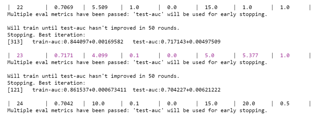
Figure 2 Bayesian Optimization Results
Part of the optimization process is shown in Figure 2. It can be seen that Bayesian optimization reached its optimal point during the 23rd iteration, with the parameters set as alpha = 4.099, column sampling ratio = 0.1, gamma = 0, maximum tree depth = 5, minimum child weight = 5.377, and subsampling ratio = 1.0, achieving the best test set AUC of 0.72.
Conclusion
This chapter provides a simple comparative analysis based on the previous chapters on ensemble learning and presents common hyperparameter tuning methods and examples. We performed a performance comparison of the three commonly used Boosting ensemble learning models: XGBoost, LightGBM, and CatBoost, using a specific data example for accuracy and speed. However, due to the specific dataset and tuning differences, the comparison results should only be used for demonstration purposes and do not genuinely represent that the LightGBM model must outperform the CatBoost model.
The three commonly used hyperparameter tuning methods are grid search, random search, and Bayesian optimization. This chapter also provides usage examples for the three hyperparameter tuning methods based on the same dataset, but due to space constraints, we did not delve deeply into the mathematical principles of each method.