Source: DeepHub IMBA


This article is about 4200 words long and is recommended to be read in over 10 minutes.
This article demonstrates the use of KNN with three different distance metrics.
The k-nearest neighbors (KNN) algorithm is a simple yet powerful algorithm that can be used for classification and regression tasks. It is easy to implement and primarily relies on different distance metrics to determine the differences between vectors. However, there are many distance metrics available, so this article demonstrates the use of KNN with three different distance metrics: Euclidean, Minkowski, and Manhattan.
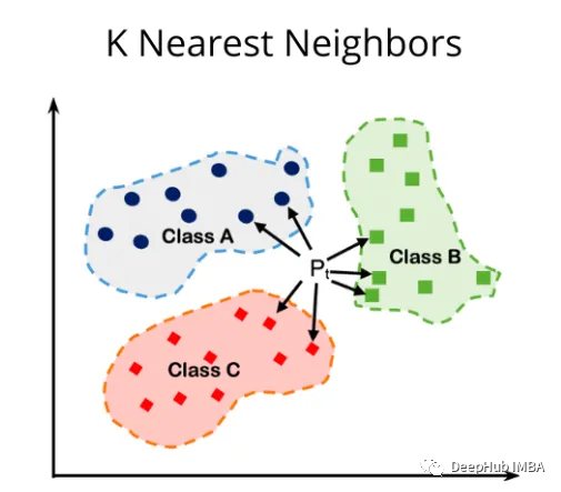
Overview of KNN Algorithm
KNN is a lazy, instance-based algorithm. It works by comparing the features of new samples with those of existing samples in the dataset. The algorithm then selects the k closest samples, where k is a user-defined parameter. The output for the new sample is determined based on the majority class of the “k” nearest samples (for classification) or the average (for regression).
There are many distance metrics available; here we select three commonly used metrics for demonstration:
def euclidean_distance(x1, x2): return math.sqrt(np.sum((x1 - x2)**2))
The euclidean_distance function calculates the Euclidean distance between two points (x1 and x2) in a multi-dimensional space. The function works as follows:
-
Subtract x2 from x1 to get the differences between the corresponding coordinates.
-
Square the differences using the **2 operation.
-
Sum the squares of the differences using np.sum().
-
Take the square root of the total using math.sqrt().
The Euclidean distance is the straight-line distance between two points in Euclidean space. By calculating the Euclidean distance, we can identify the nearest neighbors of a given sample and make predictions based on the majority class (for classification) or the average (for regression) of the neighbors. It is helpful to use Euclidean distance when dealing with continuous real-valued features, as it provides an intuitive measure of similarity.
The sum of absolute differences of the coordinates of two points.
def manhattan_distance(x1, x2): return np.sum(np.abs(x1 - x2))
The manhattan_distance function calculates the Manhattan distance between two points (x1 and x2) in a multi-dimensional space. The function works as follows:
-
Calculate the absolute differences of the corresponding coordinates using np.abs(x1 – x2).
-
Sum the absolute differences using np.sum().
Manhattan distance, also known as L1 distance or taxi cab distance, is the sum of absolute differences of the coordinates of two points. It represents the shortest path between points when movement is restricted to a grid-like structure, similar to driving a taxi on city streets.
Using Manhattan distance can be helpful when the data features have different scales or when the grid-like structure of the problem domain makes it a more suitable measure of similarity. Manhattan distance can measure the similarity or dissimilarity between samples based on their features.
Compared to Euclidean distance, Manhattan distance is less sensitive to outliers because it does not square the differences. This can make it more suitable for certain datasets or problems where the presence of outliers may significantly impact the model’s performance.
It is a generalized form of both Euclidean and Manhattan distances, parameterized by p. When p=2, it becomes Euclidean distance; when p=1, it becomes Manhattan distance.
def minkowski_distance(x1, x2, p): return np.power(np.sum(np.power(np.abs(x1 - x2), p)), 1/p)
The minkowski_distance function calculates the Minkowski distance between two points (x1 and x2) in a multi-dimensional space.
Using Minkowski distance can be helpful when you want to control the impact of differences in individual features on the overall distance. By changing the value of p, you can adjust the sensitivity of the distance measure to large or small differences in feature values, making it more suitable for specific problem domains or datasets.
Minkowski distance can measure the similarity or dissimilarity between samples based on their features. The algorithm identifies the nearest neighbors of a given sample by calculating the Minkowski distance with the appropriate p value and makes predictions based on the majority class of the neighbors (for classification) or the average (for regression).
Implementation of KNN Algorithm
Since the principle of the KNN algorithm is simple, we will implement it directly in Python, which will also provide a better understanding of the algorithm:
def knn_euclidean_distance(X_train, y_train, X_test, k):     # List to store the predicted labels for the test set     y_pred = []
     # Iterate over each point in the test set     for i in range(len(X_test)):         distances = []         # Iterate over each point in the training set         for j in range(len(X_train)):             # Calculate the distance between the two points using the Euclidean distance metric             dist = euclidean_distance(X_test[i], X_train[j])             distances.append((dist, y_train[j]))
         # Sort the distances list by distance (ascending order)         distances.sort()
         # Get the k nearest neighbors         neighbors = distances[:k]
         # Count the votes for each class         counts = {}         for neighbor in neighbors:             label = neighbor[1]             if label in counts:                 counts[label] += 1             else:                 counts[label] = 1
         # Get the class with the most votes         max_count = max(counts, key=counts.get)         y_pred.append(max_count)
     return y_pred
This ‘knn_euclidean_distance’ function is useful for solving classification problems as it can predict based on the majority class of the ‘k’ nearest neighbors. The function uses Euclidean distance as the similarity measure to identify the nearest neighbors for each data point in the test set and predict their labels accordingly. The implemented code provides an explicit method to compute distances, select neighbors, and make predictions based on the neighbors’ votes.
When using Manhattan distance, the KNN algorithm remains consistent with Euclidean distance; it only requires modifying the distance calculation function from euclidean_distance to manhattan_distance. The implementation of Minkowski distance requires an additional parameter p, as shown in the following code:
def knn_minkowski_distance(X_train, y_train, X_test, k, p):     # List to store the predicted labels for the test set     y_pred = []
     # Iterate over each point in the test set     for i in range(len(X_test)):         distances = []         # Iterate over each point in the training set         for j in range(len(X_train)):             # Calculate the distance between the two points using the Minkowski distance metric             dist = minkowski_distance(X_test[i], X_train[j], p)             distances.append((dist, y_train[j]))
         # Sort the distances list by distance (ascending order)         distances.sort()
         # Get the k nearest neighbors         neighbors = distances[:k]
         # Count the votes for each class         counts = {}         for neighbor in neighbors:             label = neighbor[1]             if label in counts:                 counts[label] += 1             else:                 counts[label] = 1
         # Get the class with the most votes         max_count = max(counts, key=counts.get)         y_pred.append(max_count)
     return y_pred
Comparison of Distance Metrics
The dataset I used is the breast cancer dataset, which can be downloaded directly from Kaggle.
This dataset is a widely used benchmark dataset in machine learning and data mining for binary classification tasks. It was collected in the 1990s by Dr. William H. Wolberg and his collaborators from the University of Wisconsin Hospital in Madison. The dataset is publicly available through the UCI Machine Learning Repository.
The Breast Cancer Wisconsin dataset contains 569 instances, each with 32 attributes. These attributes are:
ID number: A unique identifier for each sample.
Diagnosis: The target variable has two possible values – “M” (malignant) and “B” (benign).
The remaining 30 features are computed from digitized images of fine needle aspirates (FNA) of breast masses. They describe the characteristics of the nuclei in the images. Each feature is calculated for each nucleus, and then averaged to obtain 10 real-valued features:
-
Radius: The mean distance from the center to the perimeter points.
-
Texture: The standard deviation of gray-scale values.
-
Perimeter: The circumference of the nucleus.
-
Area: The area of the nucleus.
-
Smoothness: Local variation in radius lengths.
-
Compactness: Perimeter²/Area – 1.0.
-
Concavity: The severity of the contour’s concave portions.
-
Concave points: The number of concave portions of the contour.
-
Symmetry: The symmetry of the nucleus.
-
Fractal dimension: “Coastline approximation” – 1
The mean, standard error, and minimum or maximum values (the average of the three maximum values) are calculated for these ten features for each image, resulting in a total of 30 features. The dataset does not contain any missing attribute values.
Since the dataset contains 30 features, we need to perform feature selection on the dataset. The main goal of this approach is to reduce the dimensionality of the dataset by selecting a smaller subset of features that have a strong linear relationship with the target variable. By selecting highly correlated features, the aim is to maintain the predictive power of the model while reducing the number of features used, potentially improving the model’s performance and interpretability. It is important to note that this method only considers the linear relationship between features and the target variable; if the underlying relationships are non-linear or there are significant interactions between features, this method may not be effective.
Read the data and calculate the correlation:
df = pd.read_csv('/kaggle/input/breast-cancer-wisconsin-data/data.csv') corr = df.corr() corr_threshold = 0.6 selected_features = corr.index[np.abs(corr['diagnosis']) >= corr_threshold] new_cancer_data = df[selected_features]
X_train_np = np.array(X_train) X_test_np = np.array(X_test)
 # Convert y_train and y_test to numpy arrays y_train_np = np.array(y_train) y_test_np = np.array(y_test)
 k_values = list(range(1, 15)) accuracies = []
 for k in k_values:     y_pred = knn_euclidean_distance(X_train_np, y_train_np, X_test_np, k)     accuracy = accuracy_score(y_test_np, y_pred)     accuracies.append(accuracy)
 # Create a data frame to store k values and accuracies results_df = pd.DataFrame({'k': k_values, 'Accuracy': accuracies})
 # Create the interactive plot using Plotly fig = px.line(results_df, x='k', y='Accuracy', title='KNN Accuracy for Different k Values', labels={'k': 'k', 'Accuracy': 'Accuracy'}) fig.show()
 # Get the best k value best_k = k_values[accuracies.index(max(accuracies))] best_accuracy = max(accuracies) print("Best k value is:", best_k , "where accuracy is:" ,best_accuracy)
 # Run the KNN algorithm on the test set for different k and p values k_values = list(range(1, 15)) p_values = list(range(1, 6)) results = []
 for k in k_values:     for p in p_values:         y_pred = knn_minkowski_distance(X_train_np, y_train_np, X_test_np, k, p)         accuracy = accuracy_score(y_test_np, y_pred)         results.append((k, p, accuracy))
 # Create a data frame to store k, p values, and accuracies results_df = pd.DataFrame(results, columns=['k', 'p', 'Accuracy'])
 # Create the 3D plot using Plotly fig = go.Figure(data=[go.Scatter3d(     x=results_df['k'],     y=results_df['p'],     z=results_df['Accuracy'],     mode='markers',     marker=dict(         size=4,         color=results_df['Accuracy'],         colorscale='Viridis',         showscale=True,         opacity=0.8    ),     text=[f"k={k}, p={p}, Acc={acc:.2f}" for k, p, acc in results] )])
 fig.update_layout(scene=dict(     xaxis_title='k',     yaxis_title='p',     zaxis_title='Accuracy' )) fig.show()
To further improve our results, we can also scale the dataset. The main purpose of applying feature scaling is to ensure that all features have the same scale, which helps improve the performance of distance-based algorithms (like KNN). In the KNN algorithm, the distance between data points plays a crucial role in determining their similarity. If features have different scales, the algorithm may give more weight to features with larger scales, leading to suboptimal predictions. By scaling features to have a mean of zero and a unit variance, the algorithm can treat all features equally, leading to better model performance.
This article will use StandardScaler() and MinMaxScaler() to scale our dataset. StandardScaler and MinMaxScaler are two popular feature scaling techniques in machine learning. Both techniques are used to transform features to a common scale, which helps improve the performance of many machine learning algorithms, especially those that rely on distance, such as KNN or Support Vector Machines (SVM).
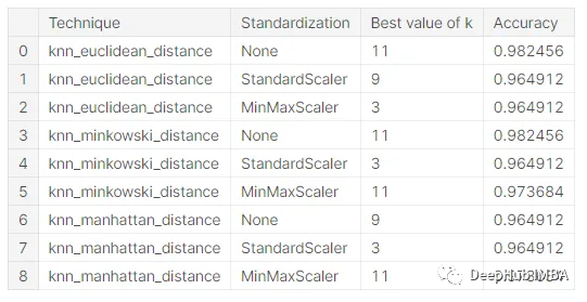
Training KNN with different scales and different distance functions allows for comparison and selection of the technique that best fits the dataset. We obtained the following results:
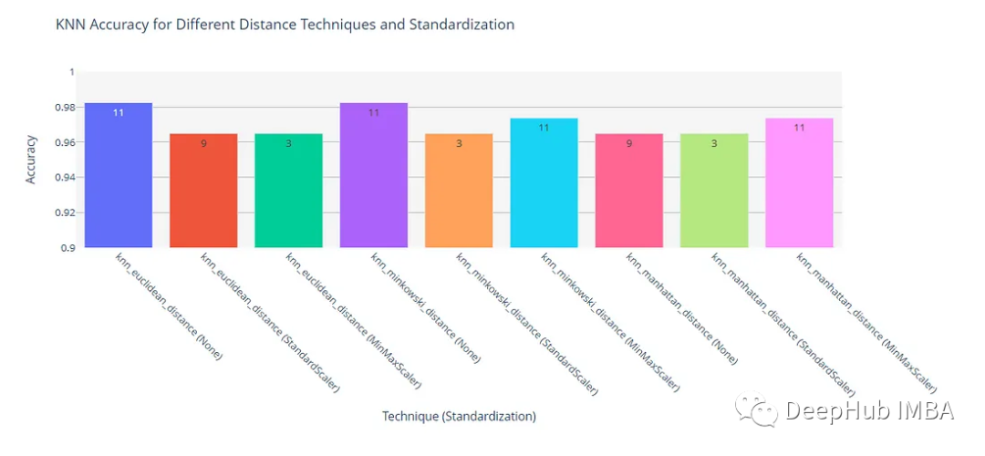
These results can be better analyzed and understood using a bar graph.
Conclusion
Based on the above results, we can draw the following conclusions:
Without feature scaling, both Euclidean distance and Minkowski distance achieved the highest accuracy of 0.982456.
Manhattan distance had relatively low accuracy in all cases, indicating that either Euclidean or Minkowski distance may be more suitable for this problem. When the value of p in the Minkowski distance measure is 2, it equals the Euclidean distance. In our experiment, the results of these two metrics were the same, confirming this is correct.
For both Euclidean and Minkowski distance measures, the highest accuracy can be achieved without any feature scaling. However, for Manhattan distance, both StandardScaler and MinMaxScaler improved the model’s performance compared to non-scaled data. This indicates that the impact of feature scaling depends on the distance measure used.
The best k value: The optimal k value depends on the distance measure and feature scaling technique. For example, k=11 is the best value when no scaling is applied and using Euclidean or Minkowski distance, while k=9 is the best value when using Manhattan distance. When feature scaling is applied, the optimal k value is usually lower, ranging from 3 to 11.
Finally, the best KNN model for this problem uses Euclidean distance measure, without any feature scaling, achieving an accuracy of 0.982456 at k=11 neighbors. This should be our best solution for this dataset when using KNN.
If you want to experiment yourself, the complete code and data can be found here:
https://www.kaggle.com/code/kane6543/knn-with-euclidean-minkowski-manhattan-distance?scriptVersionId=128083261
Author: Abdullah Siddique