Comparative Study of Transformer and RNN in Speech Applications

Original link: https://arxiv.org/pdf/1909.06317.pdf

Abstract

Sequence-to-sequence models are widely used in end-to-end speech processing, such as Automatic Speech Recognition (ASR), Speech Translation (ST), and Text-to-Speech (TTS). This paper focuses on a novel sequence-to-sequence model called the Transformer, which has achieved state-of-the-art performance in neural machine translation and other natural language processing applications. We conducted an in-depth study, comparing and analyzing the performance of the Transformer and traditional Recurrent Neural Networks (RNN) across a total of 15 ASR tasks, one multilingual ASR, one ST task, and two TTS benchmark tasks. Our experiments reveal various training techniques and the significant performance advantages achieved by the Transformer in each task, including its surprising superiority over RNNs in 13 out of 15 ASR benchmark tasks. We are preparing to release Kaldi-style reproducible recipes using open-source and publicly available datasets for all ASR, ST, and TTS tasks to enable the community to succeed based on our exciting results.

Keywords: Transformer, Recurrent Neural Network, Speech Recognition, Text-to-Speech, Speech Translation

1. Introduction

The Transformer is a sequence-to-sequence (S2S) architecture that was originally used for neural machine translation (NMT) [1] and has quickly replaced RNNs in natural language processing tasks. This paper provides an in-depth comparison of its performance in speech applications (ASR, ST, and TTS) against RNNs.

One major difficulty in applying the Transformer to speech applications is that it requires a more complex configuration than traditional RNN-based models (e.g., optimizer, network architecture, data augmentation). Our goal is to share knowledge about using Transformers for speech tasks so that the community can leverage reproducible open-source tools and recipes to fully capitalize on our exciting results.

Currently, existing Transformer-based speech applications [2]–[4] still lack open-source toolkits and reproducible experiments, whereas these resources have been provided in previous neural machine translation research [5], [6]. Therefore, we are conducting an open, community-driven project to support end-to-end speech applications using Transformers and RNNs, drawing on the success of Kaldi in the HMM-based ASR field [7]. Specifically, our experiments provide practical guidelines for tuning Transformers in speech tasks to achieve state-of-the-art results.

In our speech application experiments, we studied several aspects of the Transformer and RNN-based systems. For example, we measured word/character/regression errors against reference standards, training curves, and scalability across multiple GPUs. Contributions of this work include:

• We conducted a large-scale comparative study that contrasted the Transformer with RNNs, achieving significant performance improvements in ASR-related tasks.

• We explain the training techniques for using Transformers in speech applications (ASR, TTS, and ST).

• We provide reproducible end-to-end recipes and pre-trained models on a large number of publicly available datasets in our open-source toolkit ESPnet [8].

Related Work

Since the Transformer was initially proposed as an NMT system [1], it has been extensively studied in NMT tasks, including hyperparameter search [9], parallel implementation [5], and comparison with RNNs [10]. However, speech processing tasks in ASR [2], ST [3], and TTS [4] have only provided preliminary results. Therefore, this paper aims to gather previous foundational research and explore broader themes (e.g., accuracy, speed, training techniques) in our experiments.

2. Sequence-to-Sequence Recurrent Neural Networks

2.1 Unified Formulation of Sequence-to-Sequence

S2S (sequence-to-sequence) is a variant of neural networks that learns to convert the source sequence X into the target sequence Y [12]. In Figure 1, we present a common S2S structure used for ASR, TTS, and ST tasks. S2S consists of two neural networks: an encoder (encoder)

(1)

(2)

and a decoder

(3)

(4)

(5)

where X is the source sequence (e.g., speech feature sequence for ASR and ST or character sequence for TTS), e is the number of layers in EncBody, d is the number of layers in DecBody, and t is the index of the target frame, with all functions in the above equations implemented by neural networks. For the decoder input Y [1 : t – 1], we used a real data-based prefix during training, while a generated prefix is used during the decoding phase. During training, the S2S model learns to minimize the scalar loss value.

(6)

between the generated sequence and the target sequence.

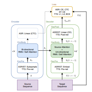Figure 1: Sequence-to-sequence architecture in speech applications

The remainder of this section describes the generic modules based on RNNs: “EncBody” and “DecBody”. We treat “EncPre”, “DecPre”, “DecPost”, and “Loss” as task-specific modules and describe them in later sections.

2.2 Recurrent Neural Network Decoder

In Equation (4), DecBody(·) generates the next target frame using the encoded sequence and the target prefix. In sequence generation, the decoder is typically unidirectional. For example, the RNN-based implementation of DecBody(·) often employs a unidirectional LSTM with an attention mechanism [13]. This attention mechanism sums the encoded source frames weighted by the source frame weights to obtain a target frame vector that is transformed along with the prefix. We refer to this type of attention as “encoder-decoder attention”.

3. Transformer

The Transformer learns sequence information through a self-attention mechanism, rather than the recurrent connections used in RNNs. This section details the self-attention-based modules in the Transformer.

3.1 Multi-Head Attention

The Transformer consists of multiple point attention layers [18].

(7)

where Q and K are the inputs to this attention layer, d is the number of feature dimensions, n is the length of Q, and m is the length of K. We refer to A as the “attention matrix”. Vaswani et al. [1] treat these inputs Q and K as queries and a set of key-value pairs, respectively.

Additionally, to enable the model to process multiple attentions in parallel, Vaswani et al. [1] extended the attention layer in Equation (7) to multi-head attention (MHA):

(8)

(9)

where V and K are the inputs to this multi-head attention layer, h is the output of the h-th attention layer, and W_h and W_o are the learnable weight matrices, with H being the number of attentions in this layer.

3.2 Self-Attention Encoder

We define the Transformer-based EncBody(·) for Equation (2), which differs from the RNN encoder in Section 2.2 as follows:

(10)

where l is the index of the encoder layer, and f is the f-th feed-forward network:

(11)

where x_t is the t-th frame of the input sequence, W is a learnable weight matrix, and b is a learnable bias vector. We refer to h_t in Equation (11) as “self-attention”.

3.3 Self-Attention Decoder

The Transformer-based DecBody(·) for Equation (4) consists of two attention modules:

(12)

where l is the index of the decoder layer. We refer to the attention matrix between the decoder input and the encoder output as “encoder-decoder attention”, similar to the attention in RNNs in Section 2.3. Since unidirectional decoders are useful in sequence generation, the attention matrix at the t-th target frame is masked to prevent connections with subsequent frames (greater than t). Masking can be performed in parallel using element-wise multiplication with a triangular binary matrix. Because it does not require sequential operations, it provides faster implementations than RNNs.

3.4 Positional Encoding

To represent temporal positions in non-recurrent models, the Transformer adopts sinusoidal positional encoding:

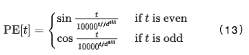
Before applying the EncBody(.) and DecBody(.) modules, the input sequence x is concatenated with p.

4. ASR Extension

In our ASR framework, the sequence-to-sequence (S2S) model predicts the target character sequence or SentencePiece [19] sequence from the input sequence (composed of speech features using log-mel filters).

4.1 ASR Encoder Architecture

In ASR, the source sequence X is represented as a sequence composed of 83-dimensional log-mel filter frames and pitch features [20]. First, EncPre(.) transforms the source sequence X into a subsampled sequence X_c using a two-layer CNN with 256 channels, a stride of 2, and a convolution kernel size of 3, similar to VGG’s max pooling [21]. Here, L is the length of the CNN output sequence. This CNN corresponds to EncPre in Equation (1). Then, EncBody transforms X_c into a series of encoded features H for the CTC and decoder networks.

4.2 ASR Decoder Architecture

The decoder network receives the encoded sequence X_e and the prefix of the target sequence Y [1:t−1], which are composed of token IDs (characters or SentencePiece [19]). First, DecPre(·) in Equation (3) embeds the tokens into learnable vectors. Next, DecBody(·) and the single linear layer DecPost(·) use X_e and Y [1:t−1] to predict the posterior distribution of the next token Y_post[t].

4.3 ASR Training and Decoding

During ASR training, the decoder and CTC modules predict the frame-wise posterior distributions of Y given the corresponding source sequence X: P_Y and P_CTC. We simply use the weighted sum of these negative log-likelihood values:

where α is a hyperparameter.

During the decoding phase, the decoder uses beam search to predict the next token given the speech features and previously predicted tokens. In beam search, the scores of S2S, CTC, and RNN language models (LM) [22] are computed as follows:

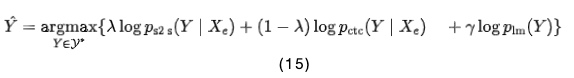
where H is a set of hypotheses for the target sequence, and λ and γ are hyperparameters.

5. ST Extension

In Speech Translation (ST), S2S receives the same source speech features and target token sequences as ASR, but the source and target languages are different. Its module definitions are the same as those in ASR. However, ST cannot cooperate with the CTC module introduced in Section 4.3 because, unlike ASR, translation tasks cannot guarantee monotonic alignment between source and target sequences [23].

6. TTS Extension

In the TTS framework, the sequence-to-sequence (S2S) model generates a series of log-mel filter features and predicts the probability of the sequence end (EOS) given the input character sequence [15].

6.1 TTS Encoder Architecture

In TTS, the input to the encoder is an ID sequence corresponding to the input characters and the EOS symbol. First, the character ID sequence is transformed into a sequence of character vectors through an embedding layer, and then a learnable scalar parameter is used to scale the vectors, to which positional encoding is added [4]. This process is the TTS implementation of EncPre(·) in Equation (1). Finally, the encoder EncBody(·) transforms this input sequence into a series of encoded features for the decoder network in Equation (2).

6.2 TTS Decoder Architecture

In TTS, the input to the decoder consists of a series of encoder features and a series of log-mel filter features. During training, the “teacher forcing” approach is used with real log-mel filter features, while during inference, an autoregressive approach is used with predicted features.

First, the target sequence of 80-dimensional log-mel filter features is transformed into a series of hidden features through Prenet [15], which is the TTS implementation of DecPre(·) in Equation (3). This network consists of two linear layers with 256 units, a ReLU activation function, and a dropout layer, followed by a projection linear layer with n units. Since the expected hidden representation from the Prenet transformation is similar to the feature space of encoder features, the Prenet helps learn a diagonal encoder-decoder attention [4]. Then, the decoder DecBody(·) in Equation (4), with an architecture identical to the encoder, transforms the encoder feature sequence and hidden feature sequence into the decoder feature sequence. For each frame of y, two linear layers are applied to compute the target features and the probability of EOS. Finally, the predicted target feature sequence is applied to Postnet [15] to predict its individual components in detail. Postnet is a five-layer CNN, where each layer is a 1D convolutional layer with 256 channels and a kernel size of 5, followed by batch normalization, a tanh activation function, and dropout. These modules are the TTS implementation of DecPost(·) in Equation (5).

6.3 TTS Training and Decoding

In TTS training, the entire network is optimized to minimize two loss functions: 1) L1 loss of the target features and 2) binary cross-entropy (BCE) loss of the EOS probability. To address the class imbalance problem in BCE calculations, a constant weight (e.g., 5) is applied to positive samples [4].

Additionally, we applied guided attention loss [24] to accelerate the learning of diagonal attention with only two heads across two layers. This is because it is known that the encoder-decoder attention matrix is only diagonal in a few heads from the target side [4]. We did not introduce any hyperparameters to balance these three loss values; we simply added them together.

During inference, the network predicts the next frame’s target features in an autoregressive manner. If the probability of EOS exceeds a certain threshold (e.g., 0.5), the network will stop predicting.

7. ASR Experiments

7.1 Datasets

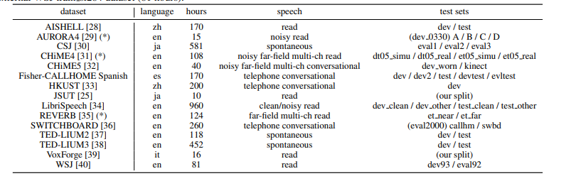Table 1: Description of ASR Datasets. The names listed in the “test set” correspond to the ASR results in Table 2. We expanded the corpus marked with (*) using the external WSJ train si284 dataset (81 hours).

7.2 Settings

We adopted the same Transformer architecture as in [41] for every corpus except the largest LibriSpeech. For RNN, we followed the optimal architectures configured for each corpus in previous studies [17], [42].

Since the training iteration speed of the Transformer is eight times that of the RNN, with finer updates, the Transformer requires different optimizer configurations than RNNs. For RNN, we adopted Adadelta [43] and the best system configuration for each corpus with early stopping strategy. For training the Transformer, we largely followed previous literature [2] (e.g., dropout, learning rate, warmup steps). In the Transformer, we did not use the development set for early stopping. We simply ran 20-200 epochs (mostly 100 epochs) and averaged the model parameters stored from the last 10 epochs as the final model.

We trained larger corpora (such as LibriSpeech, CSJ, and TED-LIUM3) on a single GPU. We also confirmed that using gradient accumulation on multiple forward/backward steps [5] to simulate multiple GPUs can achieve performances similar to those on these corpora. During the decoding phase, the Transformer and RNN share the same configurations across each corpus, such as beam search size (e.g., 20-40), CTC weight λ (e.g., 0.3), and LM weight γ (e.g., 0.3-1.0), as introduced in Section 4.3.

7.3 Results

Table 2 summarizes the ASR results for each corpus, measured by Character Error Rate (CER) and Word Error Rate (WER). The results show that in our experiments, the Transformer outperformed RNNs in 13 corpora. Although our system does not have pronunciation dictionaries, part-of-speech tagging, and data cleaning based on alignment like Kaldi, our Transformer provides comparable CER/WER to HMM-based systems Kaldi on 7 corpora. We conclude that the Transformer can even surpass end-to-end RNN-based systems and DNN/HMM-based systems in low-resource (JSUT), large-resource (LibriSpeech, CSJ), noisy (AURORA4), and far-field (REVERB) tasks. Table 3 also summarizes the results of the LibriSpeech ASR benchmark, including our results and others reported, as this is a highly competitive task. Our Transformer results are comparable to the best performances in [26], [44], [45].

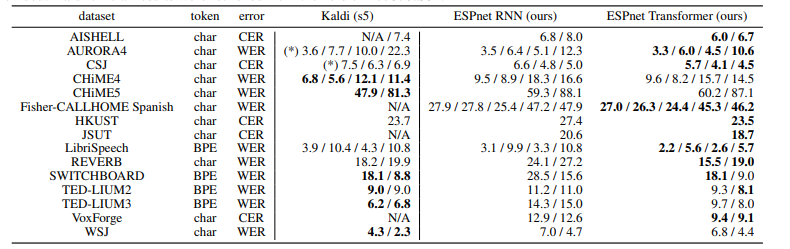Table 2: ASR results of Character/Word Error Rates. Results marked with (*) were evaluated in our environment since no official results were provided. The official results from Kaldi were extracted from version “c7876a33”.

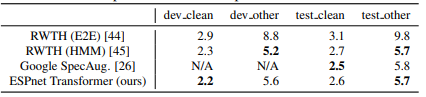Table 3: Comparison of LibriSpeech ASR benchmark results as shown in the table

Figure 2 shows the ASR training curves obtained using multiple GPUs on LibriSpeech. We observed that the accuracy of the Transformer trained with larger mini-batches is higher, while RNN does not show this trend. On the other hand, when we used smaller mini-batches for the Transformer, underfitting usually occurred after the warmup steps. In this task, the Transformer achieved comparable optimal accuracy to RNN at about eight times the speed when using a single GPU.

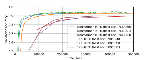Figure 2: Training curves for ASR using the LibriSpeech dataset. For each model, the mini-batch contains the maximum number of speech segments.

7.4 Discussion

We summarize the training techniques we observed in our experiments:

• When the Transformer experiences underfitting, we recommend increasing the mini-batch size, as this not only accelerates training speed but also improves accuracy, which differs from other hyperparameters.
• If multiple GPUs are not available, gradient accumulation strategies [5] can be used to simulate larger mini-batches.
• While there is no improvement in results for RNNs, using dropout is essential for the Transformer to avoid overfitting.
• We experimented with various data augmentation methods [26], [27]. They significantly improved the performance of both the Transformer and RNN.
• For RNNs, the best decoding hyperparameters γ and λ usually also apply to the Transformer.

The Transformer has some weaknesses in decoding. It is much slower than the Kaldi system due to the self-attention mechanism’s time complexity in naive implementations, where n is the length of the speech. To directly compare performance with DNN-HMM-based ASR systems, we need to develop a faster decoding algorithm for the Transformer.

8. Multilingual ASR Experiments

This section compares the performance of RNN and Transformer in ASR in a multilingual setting, considering the success of the Transformer in the previous monolingual ASR tasks. Following the method in [46], we prepared 10 different languages, including WSJ (English), CSJ (Japanese) [30], HKUST (Mandarin) [33], and VoxForge (German, Spanish, French, Italian, Dutch, Portuguese, Russian). The model is based on a single multilingual model, where the parameters are shared across all languages, and the output units include letters from all 10 languages (a total of 5,297 letters and special symbols). We used the default settings introduced in this section for both RNN and Transformer, without using RNNLM shallow fusion [21].

Figure 3 clearly shows that our Transformer significantly outperformed our RNN in 9 languages. It achieved over 10% relative improvement in 8 languages, with the largest relative improvement of 28.0% in VoxForge Italian. Compared to the RNN results in [46], which used deeper BLSTM (7 layers) and RNNLM, our Transformer still provides superior performance in 9 languages. From this result, we conclude that the Transformer also outperforms RNNs in multilingual end-to-end ASR.

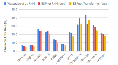Figure 3: Comparison of multilingual end-to-end ASR with RNNs by Watanabe et al. [46], ESPnet RNN, and ESPnet Transformer.

9. Speech Translation Experiments

Our baseline end-to-end ST RNN is based on [23], which is similar to the RNN structure used in our ASR system, but we did not use the convolutional LSTM layers in the original paper. The configuration of our ST Transformer is the same as that of our ASR system.

We conducted speech translation experiments on the Fisher-CALLHOME English-Spanish corpus [47]. Our Transformer improved the BLEU score from our RNN baseline of 16.5 to 17.2, applied to the “evltest” dataset of CALLHOME. During training the Transformer, we observed more severe underfitting issues than with RNNs. The solution to this problem was to use the pre-trained encoder we used in the ASR experiments, as the ST dataset contains the Fisher-CALLHOME Spanish corpus used in our ASR experiments.

10. TTS Experiments

10.1 Settings

Our baseline is the RNN-based TTS model Tacotron 2 [15]. We conducted experiments following its model and optimizer settings. We reused existing TTS recipes, including data preparation and waveform generation, which we had configured to be most suitable for RNNs. The Transformer configuration introduced in Section 3 is as follows:

10.2 Results

We compared the Transformer and RNN-based TTS using two corpora: M-AILABS [48] (Italian, 16 kHz, 31 hours) and LJSpeech [49] (English, 22 kHz, 24 hours). In the case of M-AILABS, we used an Italian male speaker (Riccardo). Figures 4 and 5 show the training curves for both corpora. From these figures, it can be seen that the Transformer and RNN provide similar results in L1 loss convergence. Similar to what was observed in ASR, we found that larger mini-batches yield better validation set L1 loss and faster training speed for the Transformer, while having a negative impact on L1 loss for RNNs. We also provide mel spectrogram samples generated in Figures 6 and 7. We conclude that the Transformer-based TTS can achieve performance levels nearly equivalent to those of RNN-based TTS.

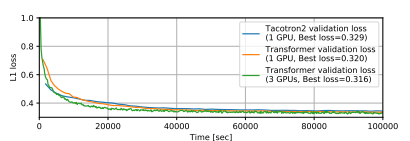Figure 4: TTS training curves on the M-AILABS dataset.Figure 5: TTS training curves on the LJSpeech dataset.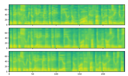Figure 6: Sample mel spectrograms on the M-AILABs dataset. (Top) Ground truth, (Middle) Tacotron 2 sample, (Bottom) Transformer sample. Input text: “E PERCHE SUBITO VIENE IN MENTE CHE ‘IDDIO NON PUO AVER FATTO UNA COSA INGIUSTA”.Figure 7: Sample mel spectrograms on the LJSpeech dataset. (Top) Ground truth, (Middle) Tacotron 2 sample, (Bottom) Transformer sample. Input text: “IS NOT CONSISTENT WITH THE STANDARDS WHICH THE RESPONSIBILITIES OF THE SECRET SERVICE REQUIRE IT TO MEET.”.

10.3 Discussion

Our experiences training the Transformer for TTS are as follows:

• If a large number of GPUs are available, using large batch training can accelerate TTS training, just like in ASR.
• For the Transformer, validation loss values, especially BCE loss, are more prone to overfitting. We recommend monitoring attention maps instead of loss values when checking for convergence.
• In the Transformer, some heads of the attention maps are not always diagonal like in Tacotron 2. Therefore, we need to choose where to apply guided attention loss [24]. Using the Transformer for decoding is also slower than using RNNs (6.5 ms per frame vs. 78.5 ms per frame on a single-threaded CPU). We also tried FastSpeech [50], which implements non-autoregressive TTS based on the Transformer. It greatly improved decoding speed (0.6 ms per frame on a single-threaded CPU) and generated speech quality comparable to autoregressive Transformers. The reduction factor introduced in [51] is also effective. It can significantly reduce training and inference time but slightly lowers quality.

In future work, we need to further explore the trade-off between training speed and quality and introduce ASR techniques (e.g., data augmentation, speech enhancement) to improve TTS systems.

11. Conclusion

We conducted a comparative study of the Transformer and RNN in speech applications, using various corpora, including ASR (15 monolingual + one multilingual), ST (one corpus), and TTS (two corpora). In the experiments of these tasks, we achieved promising results, including significant improvements in many ASR tasks, and explained how we improved the models. We believe that the reproducible recipes, pre-trained models, and training techniques described in this paper will accelerate research directions for the Transformer in speech applications.