

-
Target audience: Those who find many complex structures and layers in LLM, understand many principles, but do not know how to combine them -
This article will be long, but it should not be unnecessarily verbose -
This article may feel like a sudden blow, but it might be just right, bewildering but not overwhelming. -
Line-by-line breakdown of all operators and architecture of the LlaMa large model, including implementations of RMSNorm, ROPE, and SwiGLU -
This article does not use the huggingface library, and is implemented entirely in PyTorch, without any pre-trained models -
The starting point is the original text of “Journey to the West”, and the end point is the large model you practice creating yourself -
Prepare PyTorch; even without a GPU, it doesn’t matter, as the focus is on learning the principles of LLM, not just being able to create a new large model architecture after reading this article. -
This article will do its best to explain the principles in simple terms.
Introduction
https://colab.research.google.com/drive/1dqL8UN1UPNuEPCJzdNPbmin4vEveadgE?usp=sharing
Constructing a Simple Text Generation Model
Before constructing LlaMa, we will first build a simple seq2seq model, and then gradually add the operators RMS, Rope, and SwiGLU from LlaMa to the original Seq2seq model until we fully construct LlaMa.
First, here are some functional implementations. Although they are not very difficult, it’s best to go through them because having a mental model of the data shapes will greatly aid in understanding deep neural networks when building the model.
Importing packages
import torch
from torch import nn
from torch.nn import functional as F
import numpy as np
from matplotlib import pyplot as plt
import time
import pandas as pd
import urllib.request
These libraries will help us handle neural network models, data manipulation, visualization, timing, etc.
Creating a configuration dictionary
Define a dictionary MASTER_CONFIG to store the configuration parameters for the model:
MASTER_CONFIG = {
    # Parameters go here
}
We will update this configuration dictionary for use later.
Downloading the original text dataset of “Journey to the West”
Download the original text dataset of “Journey to the West” by Wu Cheng’en via URL and save it to the local file xiyouji.txt:
url = "https://raw.githubusercontent.com/mc112611/PI-ka-pi/main/xiyouji.txt"
file_name = "xiyouji.txt"
urllib.request.urlretrieve(url, file_name)
Reading data
Read all content from the downloaded text file:
lines = open("xiyouji.txt", 'r').read()
lines = open("xiyouji.txt", 'r').read()

# Create a simple character-level vocabulary
vocab = sorted(list(set(lines)))

# View the first n characters of the vocabulary
head_num=50
print('First {} characters of the vocabulary:'.format(head_num), vocab[:head_num])

print('Vocabulary size:', len(vocab))

# Output:
# First 50 characters of the vocabulary: ['\n', ' ', '!', '"', '#', '*', ',', '.', '—', '‘', '’', '“', '”', '□', '、', '。', '《', '》', '一', '丁', '七', '万', '丈', '三', '上', '下', '不', '与', '丑', '专', '且', '丕', '世', '丘', '丙', '业', '丛', '东', '丝', '丞', '丢', '两', '严', '丧', '个', '丫', '中', '丰', '串', '临']
# Vocabulary size: 4325
Character encoding and decoding
Map characters to numbers and vice versa so that the model can process text data:
itos = {i: ch for i, ch in enumerate(vocab)}  # index to string
stoi = {ch: i for i, ch in enumerate(vocab)}  # string to index
Next, we create a simple encoder and decoder to convert text to numbers and vice versa:
# Encoder (youth version)
def encode(s):
    return [stoi[ch] for ch in s]

# Decoder (youth version)
def decode(l):
    return ''.join([itos[i] for i in l])

# Let's test this "high-end" encoder and decoder
decode(encode("悟空"))
encode("悟空")

# Output:
# [1318, 2691]
The two output numbers represent the encoding of the characters “悟” and “空” in the vocabulary, illustrating the mapping principle.
As this is character-level encoding, not BPE or other formats of vocabulary construction, this part can be replaced with tiktoken or other mappers. The main focus here is to understand the principle, and the simpler the method used, the easier it is to understand.
# Encode the entire text into a tensor
dataset = torch.tensor(encode(lines), dtype=torch.int16)

# Check the shape, it is actually how many characters, a total of 650,000 characters
print(dataset.shape)
print(dataset)

# Output:
# torch.Size([658298])
# tensor([   0, 4319, 1694,  ...,   12,    0,    0], dtype=torch.int16)
In the code block above, we encoded the entire “Journey to the West” into a tensor. The article has over 650,000 characters, converted into a one-dimensional tensor.
Next, we build a batch
# Build batch
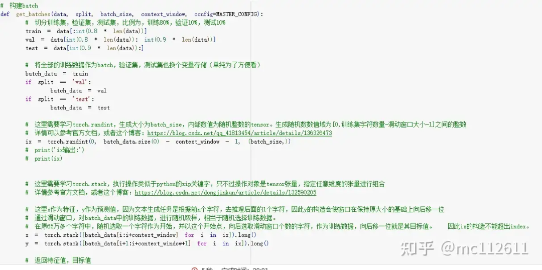
def get_batches(data, split, batch_size, context_window, config=MASTER_CONFIG):
# Split training, validation, and test sets, with a ratio of 80% training, 10% validation, 10% testing
train = data[:int(0.8 * len(data))]
val = data[int(0.8 * len(data)): int(0.9 * len(data))]
test = data[int(0.9 * len(data)):]
# Store all training data as batch, validation and test sets are also stored in different variables (just for convenience)
batch_data = train
if split == 'val':
batch_data = val
if split == 'test':
batch_data = test
# Here we need to learn torch.randint, generating a tensor of size batch_size with random integers. The generated random numbers are integers in the range [0, training set character count - sliding window size - 1]
# For details, refer to the official documentation or this blog: https://blog.csdn.net/qq_41813454/article/details/136326473
ix = torch.randint(0, batch_data.size(0) - context_window - 1, (batch_size,))
# print('ix output:')
# print(ix)
# Here we need to learn torch.stack, which executes operations similar to Python's zip keyword, but the operation object is tensor, combining specified dimensions of tensors.
# For details, refer to the official documentation or this blog: https://blog.csdn.net/dongjinkun/article/details/132590205
# Here x is the feature, y is the target value, because the text generation task is to infer the next character based on the previous n characters, thus the construction of y will shift the window one position forward.
# By sliding the window, we randomly sample from the training data in batch_data, equivalent to randomly selecting training data.
# In the original 650,000+ characters, randomly select a character as the starting point and select a number of characters equal to the sliding window size from this starting point as training data, moving one position forward makes it the target value. Therefore, ix cannot exceed index.
x = torch.stack([batch_data[i:i+context_window] for i in ix]).long()
y = torch.stack([batch_data[i+1:i+context_window+1] for i in ix]).long()
# Return feature values and target values
return x, y
torch.randint and torch.stack need to be learned; there are many articles on this.
The focus can be placed on these two lines of code:
x = torch.stack([batch_data[i:i+context_window] for i in ix]).long()
y = torch.stack([batch_data[i+1:i+context_window+1] for i in ix]).long()
Using a sliding window to obtain feature and target values, because during training, the model predicts the next character based on the previous N characters, hence the sliding window for the target value y moves one position to the right while maintaining its original size (length).
# Update the parameter dictionary based on the constructed get_batches() function.
MASTER_CONFIG.update({
    'batch_size': 8,          # No explanation
    'context_window': 16,      # Sliding window sampling, setting the sampling size
    'vocab_size':4325         # Our Journey to the West dataset contains a total of 4325 unique Chinese characters and punctuation marks
})
Construct a dictionary to store config parameters, where the sliding window value of 16 indicates that each piece of text during sampling will be divided into multiple segments of length 16. The vocab_size stated above represents the number of unique characters in the original text of “Journey to the West”, which is the size of the vocabulary.
For ease of understanding, let’s execute each function or class we construct separately to see the effect. If we pile up a lot of code, even if we execute it, seeing the final result should also be bewildering.
So we execute the get_batches function we just constructed to see the results, using the decoder (youth version) for convenience.
# Get training data
xs, ys = get_batches(dataset, 'train', MASTER_CONFIG['batch_size'], MASTER_CONFIG['context_window'])

# Since the sampling is randomly generated, we can take a look at the data, where each sampled data comes from a random starting point in the original text, each tuple being an (x,y), we can observe each x and y's first position to intuitively feel the effect of the sliding window operation
decoded_samples = [(decode(xs[i].tolist()), decode(ys[i].tolist())) for i in range(len(xs))]

print(decoded_samples)

# Output:
# [('姿娇且嫩’ !”那女子笑\n而悄答', '娇且嫩’ !”那女子笑\n而悄答道'), ('泼猢狲,打杀我也!”沙僧、八戒问', '猢狲,打杀我也!”沙僧、八戒问道'), ('人家,不惯骑马。”唐僧叫八戒驮着', '家,不惯骑马。”唐僧叫八戒驮着,'), ('著一幅“圯桥进履”的\n画儿。行者', '一幅“圯桥进履”的\n画儿。行者道'), ('从何来?这匹马,他在此久住,必知', '何来?这匹马,他在此久住,必知水'), ('声去,唿哨一声,寂然不见。那一国', '去,唿哨一声,寂然不见。那一国君'), ('刀轮剑砍怎伤怀!\n火烧雷打只如此', '轮剑砍怎伤怀!\n火烧雷打只如此,'), ('鲜。紫竹几竿鹦鹉歇,青松数簇鹧鸪', '。紫竹几竿鹦鹉歇,青松数簇鹧鸪\n')]
The output result is a list, with each element being a tuple of feature data and target values. You can observe the beginning and end of each tuple’s data to see the effect of the sliding window.
Next, we construct an evaluation function
# Construct an evaluation function
@torch.no_grad()
def evaluate_loss(model, config=MASTER_CONFIG):
    # Variable to store evaluation results
    out = {}

    # Set the model to evaluation mode
    model.eval()

    # Evaluate in both training and validation sets using the get_batches() function
    for split in ["train", "val"]:

        losses = []

        # Evaluate 10 batches
        for _ in range(10):
            # Get feature values (input data) and target values (output data)
            xb, yb = get_batches(dataset, split, config['batch_size'], config['context_window'])

            # Feed the obtained data into the model to get the loss value
            _, loss = model(xb, yb)

            # Update loss storage
            losses.append(loss.item())

        # Here is where the "train_loss" and "valid_loss" you often see in the console come from
        out[split] = np.mean(losses)

    # After evaluation, don't forget to set the model back to training mode, as it will continue training in the next epoch
    model.train()

    return out
At this point, there shouldn’t be any operations that make you feel “dazed”.
Let’s add a divider; it doesn’t serve any special purpose, but I feel that if the above content has been run through once in Jupyter or Colab without any issues, then we can continue.
As a side note, if you want to take the code and use it directly, this article may not be that magical (after all, with 650,000 words of original text from “Journey to the West”, and no pre-trained models, what kind of amazing large model can be created). If you want to learn about LLM, then I remind you once again, please read the code line by line; otherwise, it will be bewildering and mentally taxing.
Before analyzing the LlaMa architecture, we will start by creating the simplest text generation model, and then gradually add the RSM, Rope, etc., from LlaMa to this simplest text generation model. For this purpose, we will first:
Create a flawed model architecture and analyze this architecture (actually, there isn’t much analysis).
class StupidModel(nn.Module):
    def __init__(self, config=MASTER_CONFIG):
        super().__init__()
        self.config = config

        # Embedding layer, input: vocabulary size, output: dimension size
        self.embedding = nn.Embedding(config['vocab_size'], config['d_model'])

        # Create linear layers to capture feature relationships
        # Below, check if this thing is a hidden layer! The more linear layers stacked, the better! The more stacked, the greater the computational overhead!
        # The activation function used in LlaMa is SwiGLU, but here we first use Relu in this stupid model architecture
        self.linear = nn.Sequential(
            nn.Linear(config['d_model'], config['d_model']),
            nn.ReLU(),
            nn.Linear(config['d_model'], config['vocab_size']),
        )

        # This command can be memorized, or copied and pasted into your study notes. Because this line of command will directly help you see the number of parameters in the model.
        # Otherwise, you have to either calculate it by hand or listen to others talk about some model with 7B, 20B, 108B; with this command, you can directly see how many parameters your created model has
        print("Model parameters:", sum([m.numel() for m in self.parameters()]))
I think you can understand from the comments. We created a somewhat stupid model, the structure is simple: embedding, linear transformation, activation function. The only interesting thing is to remember the command below, which can be used to check the number of parameters.
print("Model parameters:", sum([m.numel() for m in self.parameters()]))
Next, we will add the forward propagation function to the above stupid model, let’s call it the “simple broken model”. In fact, broken means there is a problem. As for the problem, it will be answered shortly.
class SimpleBrokenModel(nn.Module):
    # init is the same as above, no change
    def __init__(self, config=MASTER_CONFIG):
      super().__init__()
      self.config = config
      self.embedding = nn.Embedding(config['vocab_size'], config['d_model'])
      self.linear = nn.Sequential(
          nn.Linear(config['d_model'], config['d_model']),
          nn.ReLU(),
          nn.Linear(config['d_model'], config['vocab_size']),
      )


      # Add forward propagation function
    def forward(self, idx, targets=None):
        # Instantiate the embedding layer, input maps to id data, output is the embedded data
        x = self.embedding(idx)

        # The linear layer takes the output data from the embedding layer
        a = self.linear(x)

        # Apply softmax to the linear layer output data along the last dimension to get the probability distribution
        logits = F.softmax(a, dim=-1)

        # If there are target values (which are our previous y), calculate the loss through cross-entropy loss. Reshape the output probability matrix and the target value. Unify the input and output shapes, and then calculate loss. The last dimension represents one piece of data.
        # Here you need to understand the tensor.view() function, with geometric spatial imagination to visualize the shape of the matrix.
        if targets is not None:

            loss = F.cross_entropy(logits.view(-1, self.config['vocab_size']), targets.view(-1))
            return logits, loss

        # If there is no target value, only return the result of the probability distribution
        else:
            return logits

        # Check the number of parameters
        print("Model parameters:", sum([m.numel() for m in self.parameters()]))
The comments here include both training and inference phases; the condition checks whether the target value exists. If it does not exist, only the model output is returned; if the target value exists, then the loss value is also returned.
OS: The comments were completed earlier, and I feel that there is not much left to write in this article.
# Here we set the embedding dimension of this model to 128
MASTER_CONFIG.update({
    'd_model': 128,
})

# Instantiate the model with parameters
model = SimpleBrokenModel(MASTER_CONFIG)

# Check the number of parameters again
print("Our model has this many parameters:", sum([m.numel() for m in model.parameters()]))
# Thus, we created a model with 1,128,307 parameters; feel free to modify the parameters as you wish! The computer won't explode!
We set the embedding dimension to 128; the embedding dimension of LlaMa is 4096, but we use a smaller one for training on a CPU. We get a model with 1.12 million parameters.
Next, let’s check the model output before training and the loss; the model output is just numbers, and the loss is more intuitive.
# Get training feature data and target data
xs, ys = get_batches(dataset, 'train', MASTER_CONFIG['batch_size'], MASTER_CONFIG['context_window'])

# Feed into the model to get the probability distribution matrix and loss
logits, loss = model(xs, ys)
loss

# Output:
# tensor(8.3722, grad_fn=<NllLossBackward0>)
Next, update the config hyperparameters, instantiate the model, and set the optimizer:
# Update parameters, training rounds, batch_size, and log printing interval
MASTER_CONFIG.update({
    'epochs': 1000,
    'log_interval': 10,      # Print log every 10 batches
    'batch_size': 32,
})

# Instantiate the model
model = SimpleBrokenModel(MASTER_CONFIG)

# Create an Adam optimizer, basic knowledge,
optimizer = torch.optim.Adam(
    model.parameters(),      # The optimizer optimizes all model parameters
)
Next, construct a training function and start training:
# Build a training function
def train(model, optimizer, scheduler=None, config=MASTER_CONFIG, print_logs=False):
# Loss storage
losses = []
# Record the start time of training
start_time = time.time()
# Loop through the specified number of epochs
for epoch in range(config['epochs']):
# The optimizer needs to be initialized; otherwise, each training will be based on the previous training result, leading to minimal effect
optimizer.zero_grad()
# Get training data
xs, ys = get_batches(dataset, 'train', config['batch_size'], config['context_window'])
# Forward propagation to calculate the probability matrix and loss
logits, loss = model(xs, targets=ys)
# Backward propagation to update weight parameters and learning rate optimizer
loss.backward()
optimizer.step()
# If a learning rate scheduler is provided, the learning rate will be modified by the scheduler, for example, the learning rate may change periodically, or decrease, increase; specific strategies need to be comprehensively considered for setting, details can be found by searching: lr_scheduler
if scheduler:
scheduler.step()
# Print log
if epoch % config['log_interval'] == 0:
# Training time
batch_time = time.time() - start_time
# Execute the evaluation function to calculate loss on training and validation sets
x = evaluate_loss(model)
# Store the validation loss
losses += [x]
# Print progress log
if print_logs:
print(f"Epoch {epoch} | val loss {x['val']:.3f} | Time {batch_time:.3f} | ETA in seconds {batch_time * (config['epochs'] - epoch)/config['log_interval'] :.3f}")
# Reset the start time for calculating the training time for the next round
start_time = time.time()
# Print the learning rate for the next round if a lr_scheduler is used
if scheduler:
print("lr: ", scheduler.get_lr())
# After all epochs of training are completed, print the final results
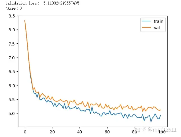
print("Validation loss: ", losses[-1]['val'])
# Return the list of loss values at each step, as we want to plot the loss over iterations
return pd.DataFrame(losses).plot()
# Start training
train(model, optimizer)
The output loss changes like this: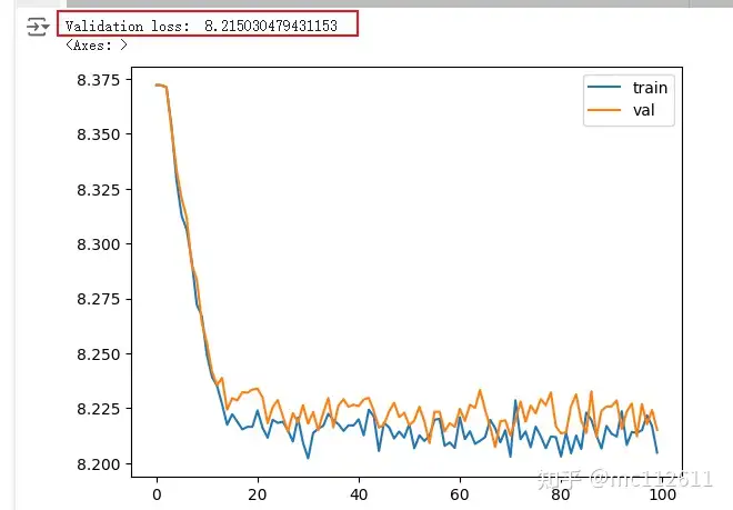 After training for 1000 epochs, the loss value decreased from 8.3722 to 8.2150!
So now you know why this model architecture is called “stupid,” or “broken.”
But! We can fix it!
First, analyze the reason:
The training framework above has some issues. Returning to the forward propagation code, in the forward() method, we used logits = F.softmax(a, dim=-1) to calculate a probability distribution on the output of the linear layer. However, the loss calculation chose cross-entropy loss, where the target value’s vocabulary mapping result is an integer while the model’s output logits is a probability matrix.
Calculating these two is like encountering a foreigner on the street in China and saying, “hey man, what’s up,” while the foreigner replies, “I can speak Chinese, what’s up?” It’s not a problem in itself, but it makes convergence a bit troublesome.
To make the loss calculation more accurate, we need to remove softmax. This ensures better calculation of cross-entropy loss.
# Remove softmax; logits should directly get the output from the last linear layer without calculating the probability distribution.
# Therefore, we rename this architecture to: not so stupid model architecture
class SimpleNotStupidModel(nn.Module):
    def __init__(self, config=MASTER_CONFIG):
      super().__init__()
      self.config = config
      self.embedding = nn.Embedding(config['vocab_size'], config['d_model'])
      self.linear = nn.Sequential(
          nn.Linear(config['d_model'], config['d_model']),
          nn.ReLU(),
          nn.Linear(config['d_model'], config['vocab_size']),
      )
      print("Model parameters:", sum([m.numel() for m in self.parameters()]))

    def forward(self, idx, targets=None):
        x = self.embedding(idx)

        # Here, the linear layer directly outputs the result without converting it to a probability matrix; only modify this part, everything else remains unchanged.
        logits = self.linear(x)
        # print(logits.shape)

        if targets is not None:

            loss = F.cross_entropy(logits.view(-1, self.config['vocab_size']), targets.view(-1))
            return logits, loss
        else:
            return logits
        print("Model parameters:", sum([m.numel() for m in self.parameters()]))
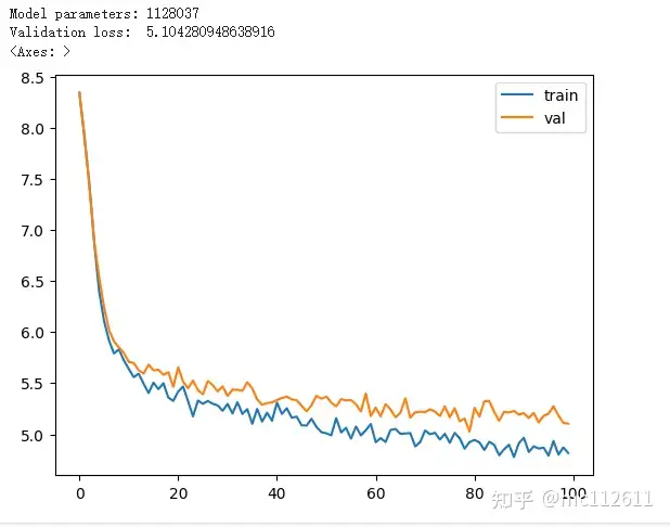
Now let’s run it again:
# Run again to instantiate various functions and start training
model = SimpleNotStupidModel(MASTER_CONFIG)
xs, ys = get_batches(dataset, 'train', MASTER_CONFIG['batch_size'], MASTER_CONFIG['context_window'])
logits, loss = model(xs, ys)
optimizer = torch.optim.Adam(model.parameters())
train(model, optimizer)
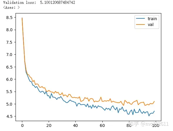
# The loss has improved significantly, dropping a lot
 Next, we construct an inference function:
We don’t plan to pass in data; in the learning version, we will just use five 0s, which represent the newline character ‘\n’, to infer the next 20 characters.
# Inference function (don’t worry too much about the output; the weights haven’t been saved, it’s just inference based on the random arrays generated during model initialization)
def generate(model, config=MASTER_CONFIG, max_new_tokens=20):
    # Generate 5 zeros as input data, representing 5 characters. This part can be replaced with other random numbers for testing.
    idx = torch.zeros(5, 1).long()
    print(idx[:, -config['context_window']:])
    for _ in range(max_new_tokens):
        # During inference, since the following n tokens depend on the previous ones, the sliding window should select the last few tokens from the input data: idx[:, -config['context_window']:]
        logits = model(idx[:, -config['context_window']:])
        # print(logits.size())
        # Get the model's output result, decode the result; here logits[:, -1, :] is quite abstract, in fact, the first dimension is the number of input characters, the second dimension is the time step, and the third dimension is the vocabulary
        # That is, for each decoding step, take the last time step's data as the output data. The decoding process is that the first decoding uses 5 tokens as input, the second decoding depends on the last four tokens of the original 5, plus one generated from the previous decoding, making it 5 tokens; this repeats.
        last_time_step_logits = logits[:, -1, :]
        # print('last_time_step_logits')
        # print(last_time_step_logits.shape)
        # Calculate the probability distribution
        p = F.softmax(last_time_step_logits, dim=-1)
        # print('p_shape')
        # print(p.shape)
        # Sample the next token based on the probability distribution using torch.multinomial
        idx_next = torch.multinomial(p, num_samples=1)
        # print('idx_next_shape')
        # print(idx_next.shape)
        # Concatenate the new idx into the decoding sequence
        idx = torch.cat([idx, idx_next], dim=-1)
    # Use the previously defined decode function to convert IDs back to characters; we obtain a 5x21 matrix of data, where each input character serves as the starting point to generate 20 characters. Since all 5 inputs are 0, which corresponds to the newline character in the vocabulary.
    print(idx.shape)
    return [decode(x) for x in idx.tolist()]

generate(model)
The output result is not surprising, as expected, quite poor:
['\n尽行者,咬道:“尽人了卖。”这人。”众僧', '\n揪啊?怎么整猜脸。”那怪教沙僧护菩萨,貌', '\n你看着国尖,不知请你。”妖王髯明。\n须行', '\n老朗哥啊,遇货出便?路,径出聋送做者,似', '\n那个急急的八戒、沙僧的树。菩萨莲削,身\n']
OK, we have constructed a simple seq2seq model. I still hope you run the code above and understand it, analyzing it line by line. If anything is unclear, print the shapes and see how the data shapes change.
If you understand everything above, we can now move on to the main topic: gradually adding the operators from LlaMa to the simple model we just built.
The code will still be annotated line by line, and in some places, I also share some thoughts for learning.
Let’s add a divider to remind ourselves: drink water, go to the bathroom, move your waist and spine, do Kegel exercises to prevent hemorrhoids. Ask yourself: Have you understood the above content thoroughly? We are about to test whether the advanced mathematics learned is solid and whether you are ready!
The main content begins:
We will add the operators from LlaMa into the simple model architecture we had earlier, mainly including:
1. RMS_Norm
2. RoPE
3. SwiGLU
Quick Understanding of RMSNorm
Norm performs normalization, which is the tensor normalization operation during the training process. By calculating the mean and variance, samples are normalized. In our university course “Probability and Statistics”, we learned that the mean of a sample represents its features, while the variance represents the degree of dispersion.
Thus, by calculating, we make the data have a mean of 0 and a variance of 1. This allows the data to follow a standard normal distribution.
Remember when the teacher emphasized this part during university: “Gaussian distribution, normal distribution”; it can also be called natural distribution, as many statistical situations in nature almost satisfy the Gaussian distribution. The numbers cluster around the center, and the further away from the center, the fewer the numbers become. The mode of the distribution is always in the middle.
Ah~ The beauty of mathematics, but it cannot compare to the beauty of advanced mathematics teachers (heh heh).
Using the mean and variance to calculate the standard deviation of the data, this retains the outliers in the data while maintaining the structure of the outliers, stabilizing gradients, reducing the problems of vanishing or exploding gradients, and also reducing overfitting issues, enhancing generalization ability.
Before RMSNorm, batch normalization was widely used, which standardizes the values of a batch of data as a sample population, calculating its mean and variance.
Then layer normalization appeared, which is a normalization process for the feature vector of each token (if you don’t know what a feature vector is, you can check my previous article on rope. You should understand the relationship between tokens and feature vectors).
RMSNorm and layer normalization’s main difference is that RMSNorm does not need to calculate both mean and variance statistics simultaneously, but only requires the calculation of the root mean square statistic. This saves 7%-64% of the computation while achieving performance almost on par with layer normalization.
RMSNorm calculation formula: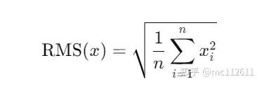
Working Principle of RMSNorm
Calculate RMS: For the input features (such as the output of neurons), first calculate its RMS value. Standardization: Divide each feature’s value by its RMS value, thus adjusting the data scale to have a mean of 0 and a standard deviation of 1.
Scaling and shifting: After normalization, RMSNorm usually introduces learnable parameters (scaling factors and biases) so that the model can learn feature representations suitable for specific tasks.
Guess: Since we are squaring and rooting, I suddenly recall the fast inverse square root algorithm that made the god of programmers — John Carmack exclaim “wow”. Of course, it’s also possible that such classic numerical computation methods have already been integrated into PyTorch.
Now that we have introduced RMSNorm, let’s implement the RMSNorm module:
class RMSNorm(nn.Module):
    def __init__(self, layer_shape, eps=1e-8, bias=False):
        super(RMSNorm, self).__init__()

        # The register_parameter() function in torch adds a parameter to the network module we created
        # Therefore, we need to add a layer that can train parameters to the RMSNorm functionality module provided by PyTorch, named scale, and initialize it as a tensor matrix with shape layer_shape, all values initialized to 1.
        self.register_parameter("scale", nn.Parameter(torch.ones(layer_shape)))

    def forward(self, x):
        # Calculate the Frobenius norm (the square sum of all elements in the matrix, then take the square root; this norm is used to measure the size of the matrix, for details please search), RMS = 1/sqrt(N) * Frobenius
        # Specifically, torch.linalg.norm(x, dim=(1, 2)) calculates the norm of x over dimensions 1 and 2. Then, the result is multiplied by x[0].numel() ** -.5. x[0].numel() represents the number of elements in the first element (i.e., the first row of x), and ** -.5 indicates taking the inverse square root.
        ff_rms = torch.linalg.norm(x, dim=(1,2)) * x[0].numel() ** -.5
        # print(ff_rms.shape)
        # Apply the ff_rms operator to the input tensor x, according to the formula, perform division; since the input vector x is three-dimensional, we need to elevate ff_rms to two dimensions to make it a three-dimensional tensor. This allows for element-wise calculations.
        raw = x / ff_rms.unsqueeze(-1).unsqueeze(-1)
        # print(raw.shape)

        # Return the normalized tensor after scaling
        # print(self.scale[:x.shape[1], :].unsqueeze(0) * raw)
        return self.scale[:x.shape[1], :].unsqueeze(0) * raw
It should be noted that the calculation raw = x / ff_rms.unsqueeze(-1).unsqueeze(-1) is performed on each element within the tensor matrix, calculating the norm (which is actually a single value, not a matrix) and dividing each element in the original input data’s tensor matrix by this normalized norm. Since RMSNorm is already inherited from PyTorch’s official nn.Module, we will make slight modifications.
Next: We will add this RMS_Norm operator to the simple model we built earlier; the code clearly shows how it was added:
class SimpleNotStupidModel_RMS(nn.Module):
    def __init__(self, config=MASTER_CONFIG):
      super().__init__()
      self.config = config
      self.embedding = nn.Embedding(config['vocab_size'], config['d_model'])
      # Here we add the RMS layer
      self.rms = RMSNorm((config['context_window'], config['d_model']))
      self.linear = nn.Sequential(
          nn.Linear(config['d_model'], config['d_model']),
          nn.ReLU(),
          nn.Linear(config['d_model'], config['vocab_size']),
      )
      print("Model parameters:", sum([m.numel() for m in self.parameters()]))

    def forward(self, idx, targets=None):
        x = self.embedding(idx)
        # Here, we add the instantiated RMS layer to take the output tensor from the embedding layer
        x = self.rms(x)

        logits = self.linear(x)
        # print(logits.shape)

        if targets is not None:
            loss = F.cross_entropy(logits.view(-1, self.config['vocab_size']), targets.view(-1))
            return logits, loss
        else:
            return logits
        # Check the number of parameters
        print("Model parameters:", sum([m.numel() for m in self.parameters()]))
After adding RMSNorm, let’s check the training effect:
# Alright, now we’ve added RMSNorm to the previous NotStupidModel, let’s execute and see
model = SimpleNotStupidModel_RMS(MASTER_CONFIG)

xs, ys = get_batches(dataset, 'train', MASTER_CONFIG['batch_size'], MASTER_CONFIG['context_window'])
logits, loss = model(xs, ys)

optimizer = torch.optim.Adam(model.parameters())

train(model, optimizer)

# The training speed noticeably accelerates after adding RMSNorm
 However, the next two operators will slow down the calculation.
Now, we will add the rotary position encoding (RoPE) to the model.
RoPE cleverly pulls the calculations of the Cartesian coordinate system into the polar coordinate space. The specific principle is quite complex; if you are interested, you can check my previous articles:
https://zhuanlan.zhihu.com/p/780744022https://zhuanlan.zhihu.com/p/830878252
We will not analyze the principles here; the main focus is on the code implementation.
I still recommend reading the above two articles, as the code part will be easy to understand.
First, we define a function to calculate the rotary position encoding:
def get_rotary_matrix(context_window, embedding_dim):
    # Initialize a zero-filled tensor with shape (context_window, embedding_dim, embedding_dim), where context_window is the number of tokens, and the last two embedding_dim form a square matrix, aligning with the attention calculation format
    R = torch.zeros((context_window, embedding_dim, embedding_dim), requires_grad=False)

    # Iterate over each token position
    for position in range(context_window):
        # Remember what I said in my previous article about features being paired? Therefore, the number of iterations is embedding_dim divided by 2
        for i in range(embedding_dim // 2):
            # Set theta, the sampling frequency, or the rotation angle; it can be divided by embedding_dim to prevent gradient issues.
            theta = 10000. ** (-2. * (i - 1) / embedding_dim)
            # Calculate the rotation angle using Euler's formula, applying sin and cos, pulling the calculation into the complex space, and applying the rotation angle to the zero-filled matrix above
            m_theta = position * theta
            R[position, 2 * i, 2 * i] = np.cos(m_theta)
            R[position, 2 * i, 2 * i + 1] = -np.sin(m_theta)
            R[position, 2 * i + 1, 2 * i] = np.sin(m_theta)
            R[position, 2 * i + 1, 2 * i + 1] = np.cos(m_theta)
            # The result obtained is the rotation position encoding matrix, but we have not yet covered the attention
    return R
Since the rotary position encoding is calculated in conjunction with the attention mechanism’s Q and K, we will first implement a single-headed attention mechanism operator:
# This is the single-headed attention mechanism
class RoPEMaskedAttentionHead(nn.Module):
    def __init__(self, config):
        super().__init__()
        self.config = config
        # Calculate Q weight matrix
        self.w_q = nn.Linear(config['d_model'], config['d_model'], bias=False)
        # Calculate K weight matrix
        self.w_k = nn.Linear(config['d_model'], config['d_model'], bias=False)
        # Calculate V weight matrix
        self.w_v = nn.Linear(config['d_model'], config['d_model'], bias=False)
        # Get the rotary position encoding matrix, which will be used to overwrite Q and K weight matrices
        self.R = get_rotary_matrix(config['context_window'], config['d_model'])


    # Here we take the function we implemented in the previous code block that creates the rotary position encoding and use it as is
    def get_rotary_matrix(context_window, embedding_dim):
        # Initialize a zero-filled tensor with shape (context_window, embedding_dim, embedding_dim), where context_window is the number of tokens, and the last two embedding_dim form a square matrix, aligning with the attention calculation format
        R = torch.zeros((context_window, embedding_dim, embedding_dim), requires_grad=False)

        # Iterate over each token position
        for position in range(context_window):
            # Remember what I said in my previous article about features being paired? Therefore, the number of iterations is embedding_dim divided by 2
            for i in range(embedding_dim // 2):
                # Set theta, the sampling frequency, or the rotation angle; it can be divided by embedding_dim to prevent gradient issues.
                theta = 10000. ** (-2. * (i - 1) / embedding_dim)
                # Calculate the rotation angle using Euler's formula, applying sin and cos, pulling the calculation into the complex space, and applying the rotation angle to the zero-filled matrix above
                m_theta = position * theta
                R[position, 2 * i, 2 * i] = np.cos(m_theta)
                R[position, 2 * i, 2 * i + 1] = -np.sin(m_theta)
                R[position, 2 * i + 1, 2 * i] = np.sin(m_theta)
                R[position, 2 * i + 1, 2 * i + 1] = np.cos(m_theta)
                # The result obtained is the rotation position encoding matrix; we have not yet covered the attention
        return R

    def forward(self, x, return_attn_weights=False):
        # The input matrix during forward propagation has the shape (batch, sequence length, dimension)

        b, m, d = x.shape  # batch size, sequence length, dimension

        # Linear transformations for Q, K, V
        q = self.w_q(x)
        k = self.w_k(x)
        v = self.w_v(x)

        # Apply the rotary position encoding to Q and K, where torch.bmm performs the outer product on matrices, and transpose transposes the Q matrix, applying the rotary position encoding to it before transposing back to its original shape.
        # Considering the length of the input text, we truncate the position encoding matrix along the first dimension if it is too long.
        q_rotated = (torch.bmm(q.transpose(0, 1), self.R[:m])).transpose(0, 1)
        # Similarly, apply the rotary position encoding to K
        k_rotated = (torch.bmm(k.transpose(0, 1), self.R[:m])).transpose(0, 1)

        # Scale the attention mechanism's dot product to prevent the attention tensor from becoming too long, which can cause gradient explosion.
        activations = F.scaled_dot_product_attention(
            q_rotated, k_rotated, v, dropout_p=0.1, is_causal=True
        )
        # If return_attn_weights is set to 1, we need to mask the attention, as during learning, we hope the model can predict the token based on the previous n tokens, rather than an open-book exam.
        if return_attn_weights:
            # Create an attention mask matrix, where the torch.tril function takes the lower triangle of the matrix, setting the rest to 0
            attn_mask = torch.tril(torch.ones((m, m)), diagonal=0)
            # Calculate the attention weights matrix, normalizing along the last dimension (check why it's the last dimension! Because the last dimension is the feature vector of each token!)
            attn_weights = torch.bmm(q_rotated, k_rotated.transpose(1, 2)) / np.sqrt(d) + attn_mask
            attn_weights = F.softmax(attn_weights, dim=-1)
            return activations, attn_weights

        return activations
The single-headed attention mechanism has been implemented; now let’s implement the multi-headed attention mechanism:
# The single-headed attention mechanism has been implemented; now we will implement the multi-headed attention mechanism
class RoPEMaskedMultiheadAttention(nn.Module):
    def __init__(self, config):
        super().__init__()
        self.config = config
        # An attention head object has been created; for multi-head, we first create this object multiple times. Generate multiple attention heads and store them in a list.
        self.heads = nn.ModuleList([
            RoPEMaskedAttentionHead(config) for _ in range(config['n_heads'])
        ])
        # In the model structure, create a linear layer (hidden layer) to linearly output the tensor matrix from the attention head, seeking features among multiple heads. More importantly, after multiple heads calculate attention, the shape of the tensor matrix changes, so we create a linear layer to return the tensor matrix to the original input shape.
        # To prevent overfitting, a dropout layer is used with a rate of 0.1.
        # The input shape of the linear layer: the number of attention heads multiplied by the dimension of the matrix, related to my previous article on the key matrix, sharing weights among multi-heads to reduce computation.
        self.linear = nn.Linear(config['n_heads'] * config['d_model'], config['d_model'])
        self.dropout = nn.Dropout(0.1)

    def forward(self, x):
        # The input matrix shape x: (batch, sequence length, dimension)

        # Each attention mechanism head processes X for computation. (This part may speed up with parallel execution, but I’m unsure if PyTorch automatically calls parallel processing)
        heads = [h(x) for h in self.heads]
        # The input tensor x undergoes multiple heads to compute attention (also, the attention has already been overwritten by RoPE), re-concatenated into a new matrix and stored back into variable x. You should feel that the matrix shape has changed by now.
        x = torch.cat(heads, dim=-1)

        # This is where the linear layer comes into play
        x = self.linear(x)

        # Randomly drop out some neurons to prevent overfitting
        x = self.dropout(x)
        return x
If you have already felt bewildered and mentally taxed, it is still a good idea to learn about the principle of RoPE; even if it’s not from my articles, you can find some understandable articles, explanations in layman’s terms, or even ask ChatGPT. Any method that aligns the author’s narrative style with your brainwave frequency so that you can understand is fine.
Alright, we have implemented the above functions; let’s update the config hyperparameter dictionary to set the number of attention mechanism heads. LlaMa has 32 attention heads, but we will create 8:
MASTER_CONFIG.update({
    'n_heads': 8,
})
Next, we will update our suggested model, which previously included RMS_Norm, and this time we will add the multi-headed attention mechanism with ROPE position encoding!
# Now we have created all the operators: RMS, ROPE, SWIGLU; let’s build our LlaMa! First, we implement the LlaMa functional block, then stack them.
# There’s not much to explain about the functionality; if you have carefully read up to here, every line of code below should be easy for you.
class RopeModel(nn.Module):
    def __init__(self, config):
        super().__init__()
        self.config = config

        # Embedding layer
        self.embedding = nn.Embedding(config['vocab_size'], config['d_model'])

        # RMSNorm layer
        self.rms = RMSNorm((config['context_window'], config['d_model']))

        # Rotary position encoder + attention mechanism
        self.rope_attention = RoPEMaskedMultiheadAttention(config)

        # Linear layer + activation function for nonlinear output!
        self.linear = nn.Sequential(
            nn.Linear(config['d_model'], config['d_model']),
            nn.ReLU(),
        )

        # Final output because we need to decode, the dimension of the output must match the vocabulary size!
        self.last_linear = nn.Linear(config['d_model'], config['vocab_size'])

        print("model params:", sum([m.numel() for m in self.parameters()]))
    # Forward propagation
    def forward(self, idx, targets=None):
        # embedding, no need to explain
        x = self.embedding(idx)
        # Normalize values, no need to explain
        x = self.rms(x)
        # Add, let me explain, because attention needs to overwrite the original matrix, imagine two matrices of the same shape like two sheets of paper; the left hand has one sheet, the right hand has another, they overlap by adding! Using addition means adding the elements of the two matrices based on their positions!
        x = x + self.rope_attention(x)
        # Normalize again!
        x = self.rms(x)
        # Because directly computing the normalized value may cause gradient issues, we use the normalized value as a correction factor to overwrite!
        x = x + self.linear(x)
        # Finally, we output the neuron output corresponding to the vocabulary quantity!!!!
        logits = self.last_linear(x)

        # During training, there are target values
        if targets is not None:
            loss = F.cross_entropy(logits.view(-1, self.config['vocab_size']), targets.view(-1))
            return logits, loss
        # During validation or inference, there are no target values; only return results
        else:
            return logits
Let’s check the hyperparameter dictionary:
# Check our hyperparameter dictionary
MASTER_CONFIG

# Output:
#{'batch_size': 32,'context_window': 16, 'vocab_size': 4325,'d_model': 128,'epochs': 1000,'log_interval': 10,'n_heads': 8,'n_layers': 4}
Let’s test whether the created functional block has any issues:
# Using the config dictionary, create the llama functional block
block = LlamaBlock(MASTER_CONFIG)

# Generate a random data and feed it into this llama functional block to see if there are bugs
random_input = torch.randn(MASTER_CONFIG['batch_size'], MASTER_CONFIG['context_window'], MASTER_CONFIG['d_model'])

# Execute and see the output
output = block(random_input)
output.shape
Now we assemble LlaMa!
# Now, we assemble LlaMa
from collections import OrderedDict
class Llama(nn.Module):
    def __init__(self, config):
        super().__init__()
        self.config = config
        # Embedding, no explanation
        self.embeddings = nn.Embedding(config['vocab_size'], config['d_model'])
        # According to the passed stacking layer count, create Llama functional blocks. Note that OrderedDict is a special type of dictionary that preserves the order of insertion, with earlier inserted data appearing first.
        # Here, we will stack 4 layers of Llama functional blocks
        self.llama_blocks = nn.Sequential(
            OrderedDict([(f"llama_{i}", LlamaBlock(config)) for i in range(config['n_layers'])])
        )
        # FFN layer, including: linear layer, activation function for nonlinear transformation, and then a linear layer to output the final decoding value.
        self.ffn = nn.Sequential(
            nn.Linear(config['d_model'], config['d_model']),
            SwiGLU(config['d_model']),
            nn.Linear(config['d_model'], config['vocab_size']),
        )

        # Check how many parameters our large model has!
        print("model params:", sum([m.numel() for m in self.parameters()]))

    def forward(self, idx, targets=None):
        # embedding
        x = self.embeddings(idx)
        # Llama model calculation
        x = self.llama_blocks(x)
        # FFN calculation to obtain logits
        logits = self.ffn(x)

        # No target values during inference, only return results
        if targets is None:
            return logits
        # During training, there are target values, need to output results and loss for backpropagation to update weights!
        else:
            loss = F.cross_entropy(logits.view(-1, self.config['vocab_size']), targets.view(-1))
            return logits, loss
Let’s train LlaMa:
# Start training our Llama
llama = Llama(MASTER_CONFIG)
xs, ys = get_batches(dataset, 'train', MASTER_CONFIG['batch_size'], MASTER_CONFIG['context_window'])
logits, loss = llama(xs, ys)
optimizer = torch.optim.Adam(llama.parameters())
train(llama, optimizer)
Let’s infer:
# Let’s see the inference effect (actually there isn’t much effect -.-)
# Don’t forget that the input data in generate is the 5 zeros we created; if replaced with the encoded numbers, it’s also fine! Form a list, convert to tensor, this should be no problem right?
generated_text = generate(llama, MASTER_CONFIG, 500)[0]
print(generated_text)
The inference effect is still quite abstract. It feels like practicing the “Xinhua Dictionary” in reverse.
Of course, we never expected the inference effect to be good. That’s why I said earlier that this article itself isn’t plug-and-play; it’s more suitable for Chinese babies learning about large models.
玄兔春非朦意敖叶祥肤水沉岭日疼清赛。萝范燕旗顺清气瑜灵子庄。海藏御直熟列棱
尉火牙心正花,四位幸堂国如生岖。
辟两只道:千人人纵开羊堤进宝贝,乃人头破马前立阵,腰一年心;足如蜻丛杨馥新一耸飘木
膜须寺颜凤丹叶獐绦;桃送?
添牛福芽蟒菜丛体茵岁鹅宫丰,贼培莲豆龙东兵,九千
蓝穿鸣人罔二无团蛇陌盔,日滚听拿
万盏可帮迎。这壁楼去常路递淫栖询除朱,
渎制然便跑神果。因安群猴俱无发能放。今
钟无削乐都有僵拿,
能可怕饭息饯?”又说他怒道:“师父是两魔头请久得五条大神神净,全
天
前顷飞影多功。有四尺阳皆之挨初山,只然艰薤盘裳见大仙的清过武前,阻雨野轮板雕青应沫。
月海依乃射仙僧岸,更天淡海月蓬为白巅耀院,日花匾盏神润晴涧攒肾壑笠绵,恶非狐成聚三藏灵玉火花,玉西草奇竹主深。
德太影任涨青叶,十莲缨猪大圣天寸耀亮红、平
啸壮名空猿携绩蝶泾帝妖
满冻在我跑旧热力。唬得小子,
又五凤景晚。细抖见出前蓝泛卿西浪花白帘谷琶?一张酥罢旨
严胜锁来鬼处将他几个人师父!”喝道:“我们这厮伏:“可来,我伤得!不要说,有水洒悭迟。
待吾叫做,
俱的劈摆道者怕形,等我个妖精坐在鹤下,钩怪藏
手里罩放发,
天篮,掣身
Let’s run the test set as well; I even forgot about the test set, right? If you forgot, take a look at the get_batch function:
# Now let’s run the test set
# Get the feature values and target values of the test set
xs, ys = get_batches(dataset, 'test', MASTER_CONFIG['batch_size'], MASTER_CONFIG['context_window'])

# Feed into Llama to get the loss
logits, loss = llama(xs, ys)

print(loss)
# Output:
# tensor(4.7326, grad_fn=<NllLossBackward0>)
Let’s add some features to make it look more professional by adding a learning rate scheduler
# There are still optimization points, don’t forget the optimizer! And the learning rate scheduler!
# Adjust parameters and come again!

MASTER_CONFIG.update({
    "epochs": 1000
})

# Choose cosine annealing for the learning rate optimizer
llama_with_cosine = Llama(MASTER_CONFIG)

llama_optimizer = torch.optim.Adam(
    llama.parameters(),
    betas=(.9, .95),
    weight_decay=.1,
    eps=1e-9,
    lr=1e-3
)
# The cosine annealing learning rate optimizer gradually reduces the learning rate, reaching the lowest value at the end. For details, you can search; there are many articles on this.
scheduler = torch.optim.lr_scheduler.CosineAnnealingLR(llama_optimizer, 300, eta_min=1e-5)

# Run it!
train(llama_with_cosine, llama_optimizer, scheduler=scheduler)
 Running for 20,000 epochs is sufficient. After all, all parameters are set randomly…
Alright, that’s basically it. We have the main structure now; the remaining strategies or adding other operators can follow the structure. There’s nothing we can’t do. The focus can be on the input and output. Matrix calculations require mathematical knowledge to distinguish between element-wise calculations and overall vector-matrix calculations.
If you have understood the content above, then I believe the model.py file in the llama3 source code can be easily handled. I have to say, the Meta team really wants the whole world to understand their code; it’s highly organized and explanatory, making it very suitable for learning about large models.
https://github.com/meta-llama/llama3/blob/main/llama/model.py
I left a little trick in the shared Colab notebook; it’s not really a trick, just deploying the artificial intelligence we just created using FastAPI as an asynchronous processing service. If you’re not interested, you can skip it.

Scan the QR code to add the assistant on WeChat
About Us