BP Neural Network Algorithm and Practice

Source: CodeMeals

cnblogs.com/fengfenggirl/p/bp_network.html

Neural networks were once very popular, went through a period of decline, and are now gaining popularity again due to deep learning. There are many types of neural networks: feedforward networks, backpropagation networks, recurrent neural networks, convolutional neural networks, etc. This article introduces the basic backpropagation neural network (BP), focusing on the basic algorithm flow and some personal experiences in training BP neural networks.

Structure of BP Neural Network

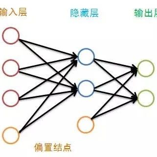
A neural network simulates the working method of the brain’s neural units but is greatly simplified. The neural network consists of many layers, with each layer containing numerous units. The first layer is called the input layer, the last layer is the output layer, and the intermediate layers are called hidden layers. In a BP neural network, only adjacent neural layers have connections between their units, and every layer, except for the output layer, has a bias node:

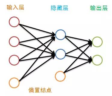
Although only one hidden layer is drawn in the figure, there is no limit to the number of layers. Traditional neural network learning experience suggests that one layer is sufficient, but recent deep learning approaches do not agree. The bias node is used to represent features not present in the training data. The bias node generates different biases for each node in the next layer based on the different weights assigned to it, so we can consider the bias as an attribute of each node (except for the input layer). We omit the bias nodes in the diagram:

Before describing the training of the BP neural network, let’s take a look at the attributes of each layer of the neural network:

1. Each neural unit has a certain amount of energy, defined as the output value Oj of node j;

2. The connections between nodes in adjacent layers have a weight Wij, which ranges from [-1,1];

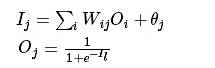
3. Each node in every layer (except the input layer) has an input value, which is the sum of the energies from all nodes in the previous layer weighted by their respective weights plus the bias;

4. Each layer (except the input layer) has a bias value, which ranges from [0,1];

5. The output value of each node (except the input layer) is a nonlinear transformation of that node’s input value;

6. We assume that the input layer has no input values, and its output values are the attributes of the training data. For example, for a record X=<(1,2,3), category 1>, the output values of the three nodes in the input layer are 1, 2, and 3, respectively. Therefore, the number of nodes in the input layer generally equals the number of attributes in the training data.

Training a BP neural network essentially involves adjusting the weights and biases of the network, and the training process consists of two parts:

1. Forward propagation, where output values are passed layer by layer;

2. Backward feedback, where weights and biases are adjusted layer by layer in reverse;

Let’s first look at forward propagation.

Forward Propagation (Feed-Forward)

Before training the network, we need to randomly initialize the weights and biases, taking a random real number for each weight in the range of [-1,1] and a random real number for each bias in the range of [0,1]. After that, we start forward propagation.

The training of a neural network is completed through multiple iterations, where each iteration uses all records in the training set, but each training step only uses one record. The abstract description is as follows:

while the termination condition is not met:

for record:dataset:

trainModel(record)

First, we set the output values of the input layer. Assuming the number of attributes is 100, we set the number of neural units in the input layer to 100, with each node Ni of the input layer corresponding to the attribute value xi of the record at dimension i. The operation for the input layer is that simple; the operations for the other layers are a bit more complex. For layers other than the input layer, the input value is the weighted sum of the previous layer’s input values plus the bias, and the output value of each node is a transformation of its input value.

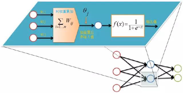
The calculation process for the output layer during forward propagation is as follows:

For each node in the hidden and output layers, we calculate the output value as shown in the diagram above, completing the forward propagation process, followed by backward feedback.

Backward Feedback (Backpropagation)

Backward feedback starts from the last layer, which is the output layer. The purpose of training the neural network for classification is often to ensure that the output of the last layer can describe the category of the data record. For example, in a binary classification problem, we often use two neural units as the output layer. If the output value of the first neural unit in the output layer is greater than that of the second, we consider the data record belongs to the first category; otherwise, it belongs to the second category.

Remember that during our first forward propagation, all the weights and biases of the network were randomly initialized, so the output of the network could not yet describe the categories of the records. Therefore, we need to adjust the network parameters, namely the weights and biases, based on the difference between the output values of the output layer and the actual categories. The optimization goal of the neural network is to minimize this difference. For the output layer:

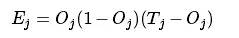
Where Ej represents the error value of the j-th node, Oj represents the output value of the j-th node, and Tj records the target output value. For a binary classification problem, we use 01 to represent class 1 and 10 to represent class 2. If a record belongs to class 1, then T1=0 and T2=1.

The intermediate hidden layers do not directly interact with the data record categories but compute their errors by summing the errors of all nodes in the next layer, as follows:

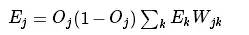
Where Wjk represents the weight from the j-th node in the current layer to the k-th node in the next layer, and Ek is the error rate of the k-th node in the next layer.

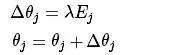
After calculating the error rates, we can update the weights and biases using these error rates, starting with the weight updates:

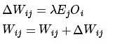
Where λ represents the learning rate, which takes values from 0 to 1. A larger learning rate allows for faster convergence but may lead to local optima, while a smaller learning rate slows convergence but can gradually approach the global optimum.

After updating the weights, there is one last parameter to update, which is the bias:

Thus, we have completed one training process for the neural network. By continuously using all data records for training, we can obtain a classification model. The iterations cannot go on indefinitely; there must be a termination condition.

Training Termination Conditions

Each round of training uses all records from the dataset, but when to stop? The termination conditions are as follows:

1. Set a maximum number of iterations, for example, stop training after 100 iterations over the dataset.

2. Calculate the prediction accuracy of the training set on the network, and stop training once a certain threshold is reached.

Using BP Neural Network for Classification

I wrote a BP neural network and tested it on the MNIST handwritten digit recognition dataset. The MNIST dataset contains 12,000 training images and 20,000 test images, each image being a 28×28 grayscale image. I binarized the images, and the neural network parameters were set as follows:

1. Input layer set to 28*28=784 input units;

2. Output layer set to 10, corresponding to 10 digit categories;

3. Learning rate set to 0.05;

After about 50 iterations, I achieved a 99% accuracy on the training set, and a 90.03% accuracy on the test set. The improvement space for a simple BP neural network is limited, but someone on Kaggle has already achieved a 99.3% accuracy on the test set using a convolutional neural network. The code was written in C++ last year and has a strong JAVA flavor; its value is not significant, but the comments are quite detailed. You can check it out here. Recently, I wrote a Java multithreaded BP neural network, but it’s not convenient to share it now. If the project fails, I’ll make it available later.

Some Experiences in Training BP Neural Networks

Here are some personal experiences in training neural networks:

1. The learning rate should not be set too high, generally less than 0.1. Initially, I set it to 0.85, but the accuracy could not improve, indicating that it was clearly trapped in a local optimum;

2. Input data should be normalized. I initially tested with 0-255 grayscale values, which did not perform well. After converting to binary (0-1), the performance improved significantly;

3. Data records should ideally be randomly distributed; do not sort the dataset by records. For instance, if there are 10 categories in the dataset and we sort it by category and train the neural network record by record, the model will only remember the most recently trained category and forget the earlier ones;

4. For multi-class problems, such as Chinese character recognition, there are over 7000 commonly used characters, meaning there are 7000 categories. If we set the output layer to 7000 nodes, the computation will be enormous, and the parameters will be too many to converge easily. In this case, we should encode the categories; 7000 Chinese characters can be represented with just 13 binary bits, so we only need to set 13 nodes in the output layer.

References:

Jiawei Han. “Data Mining Concepts and Techniques”