Source: DeepHub IMBA



This article is about 3300 words, suggested reading time is 10 minutes.
This article will introduce the BiTCN model, which utilizes two Temporal Convolutional Networks (TCN) to encode past and future covariates while maintaining computational efficiency.

In the field of time series forecasting, model architecture often relies on Multi-Layer Perceptron (MLP) or Transformer architectures.

MLP-based models, such as N-HiTS, TiDE, and TSMixer, can achieve very good prediction performance while maintaining fast training. Transformer-based models, such as PatchTST and ITTransformer, have also achieved good performance but require more memory and time to train.

There is one architecture that remains underutilized in forecasting: Convolutional Neural Networks (CNN). CNNs have been applied in computer vision, but their application in forecasting is still limited, with TimesNet being a recent example. However, CNNs have been shown to be effective in handling sequential data, and their architecture allows for parallel computation, which can greatly speed up training.

In this article, we will detail BiTCN, a model proposed in March 2023 in the paper “Parameter-efficient deep probabilistic forecasting”. By utilizing two Temporal Convolutional Networks (TCN), this model can encode past and future covariates while maintaining computational efficiency.

BiTCN

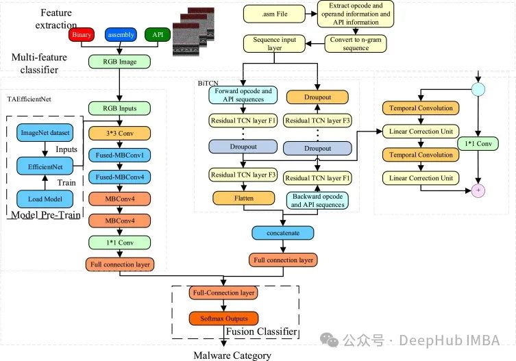
BiTCN uses two Temporal Convolutional Networks, hence the name BiTCN. One TCN is responsible for encoding future covariates, while the other is responsible for encoding past covariates and historical values of the sequence. This allows the model to learn temporal information from the data, and the use of convolution maintains computational efficiency.

Let’s take a closer look at its architecture. The structure of BiTCN consists of many temporal blocks, each of which consists of:

An dilated convolution, a GELU activation function, followed by dropout, and finally a fully connected layer.

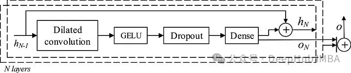
As shown in the figure above, each temporal block produces an output o, and the final prediction is the sum of all outputs from each block across N layers.

While dropout layers and fully connected layers are common components in neural networks, we will detail dilated convolutions and the GELU activation function.

Dilated Convolution

To better understand the purpose of dilated convolution, let’s review how standard convolution works.

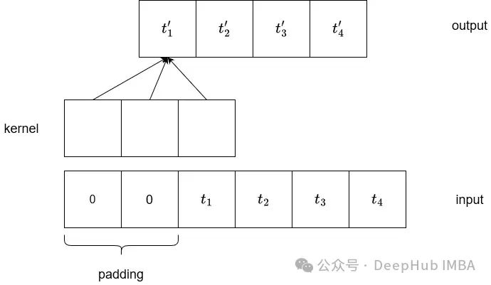
In the figure above, we can see a typical convolution of one-dimensional input. The input sequence is zero-padded on the left to ensure the output length is the same.

If the kernel size is 3 and the stride is 1, then the length of the output tensor is also 4.

We can see that each output element depends on three input values. That is, the output depends on the value at the index and the two preceding values.

This is what we refer to as the receptive field. Since we are dealing with time series data, increasing the receptive field would be beneficial, allowing the output computation to consider a longer history.

We can simply increase the kernel size or stack more convolutional layers. However, increasing the kernel size is not the best option, as it may lose information, and the model may not learn useful relationships in the data. So how about stacking more convolutions?

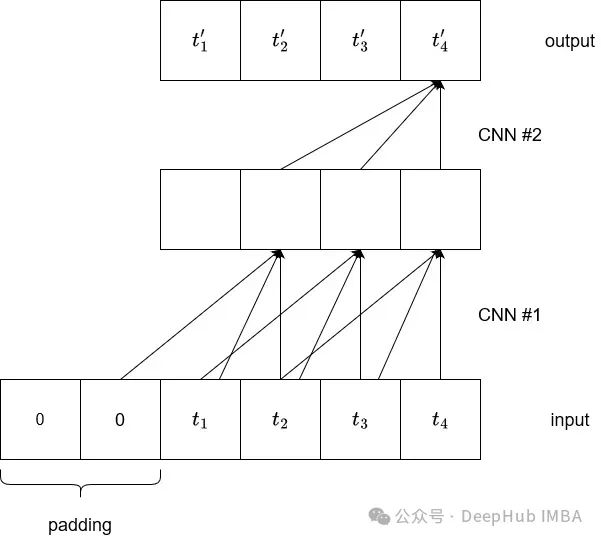
We can see that by stacking two convolutions with a kernel size of 3, the last output element now depends on five input elements, increasing the receptive field from 3 to 5.

However, increasing the receptive field in this way would lead to a very deep network, which is where dilated convolutions come in, as they can increase the receptive field while avoiding adding too many layers to the model.

In the figure above, we can see the result of running dilated convolution. Each two elements generate one output. Therefore, we can see that we now have 5 receptive fields without having to stack convolutions.

To further increase the receptive field, we stack many dilated kernels with a dilation rate (usually set to 2). This means the first layer will have a kernel with a dilation of 2¹, then a kernel with a dilation of 2², and so on.

This allows the model to consider longer input sequences to generate outputs. By using the dilation rate, a reasonable number of layers can be maintained.

GELU Activation Function

Many deep learning architectures adopt the ReLU activation function.

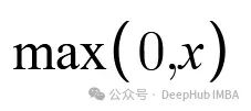
We can see that ReLU simply takes the maximum between 0 and the input. That is, if the input is positive, it returns the input. If the input is negative, it returns zero.

While ReLU helps alleviate the vanishing gradient problem, it also leads to what is known as the “Dying ReLU” problem. This occurs when certain neurons in the network output only 0, meaning they no longer contribute to the learning of the model. To address this, we can use GELU.

With this function, when the input is less than zero, the activation function allows small negative values.

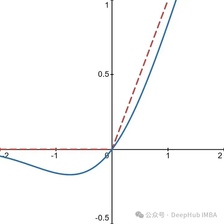
This way, neurons are less likely to die out, as non-zero values can be returned with negative inputs. This provides a richer gradient for backpropagation, allowing us to maintain the integrity of the model’s capabilities.

Complete Architecture of BiTCN

Now that we understand the inner workings of the temporal blocks in BiTCN, let’s see how they are combined in the model.

In the figure above, we can see that lagged values are combined with all past covariates before passing through the dense layer and temporal block stack.

We also see that categorical covariates are embedded first, and then combined with other covariates. Here, past and future covariates are combined together, as shown below. The output is a combination of information from lagged values and covariates, as shown below.

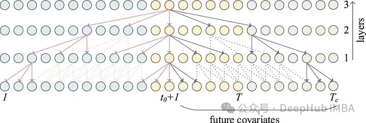
The blue points in the figure above represent the input sequence, the yellow points represent the output sequence, and the red points represent future covariates. We can see how the forward-looking temporal blocks with dilated convolutions help inform the output by processing information from future covariates.

Finally, BiTCN uses the Student’s t-distribution to construct confidence intervals around the predictions.

Using BiTCN for Forecasting

Next, we will apply BiTCN alongside N-HiTS and PatchTST for a long-term forecasting task.

We will use it to predict the daily views of a blog website. The dataset contains daily views as well as exogenous features such as indicators of new article publication dates and holidays in the United States.

We use the neuralforecast library, as it is the only library that provides a ready-to-use implementation of BiTCN that supports exogenous features. The code and data for this article will be provided at the end.

 import pandas as pd import numpy as np import matplotlib.pyplot as plt
 from neuralforecast.core import NeuralForecast from neuralforecast.models import NHITS, PatchTST, BiTCN

Load the data into a DataFrame.

df = pd.read_csv('https://raw.githubusercontent.com/marcopeix/time-series-analysis/master/data/medium_views_published_holidays.csv') df['ds'] = pd.to_datetime(df['ds'])

Let’s take a look at the data:

 published_dates = df[df['published'] == 1] holidays = df[df['is_holiday'] == 1]
 fig, ax = plt.subplots(figsize=(12,8))
 ax.plot(df['ds'], df['y']) ax.scatter(published_dates['ds'], published_dates['y'], marker='o', color='red', label='New article') ax.scatter(holidays['ds'], holidays['y'], marker='x', color='green', label='US holiday') ax.set_xlabel('Day') ax.set_ylabel('Total views') ax.legend(loc='best')
 fig.autofmt_xdate()
 plt.tight_layout()

We can clearly see the weekly seasonality, with more views on weekdays than on weekends.

Traffic peaks are often accompanied by the release of new articles (indicated by red dots), as new content usually drives more traffic. Lastly, the US holidays (marked by green crosses) typically mean lower traffic.

So we can determine that this is a dataset significantly affected by exogenous features, which makes it a great use case for BiTCN.

Data Processing

We will split the data into training and testing sets. We will keep the last 28 entries for testing.

train = df[:-28] test = df[-28:]

Then, we create a DataFrame containing the dates for the prediction range, along with future values for the exogenous variables.

Providing future values for the exogenous variables makes sense, as future US holiday dates are known in advance, and article releases can also be planned.

future_df = test.drop(['y'], axis=1)

Modeling

In this project, we will use N-HiTS (based on MLP), BiTCN (based on CNN), and PatchTST (based on Transformer).

N-HiTS and BiTCN both support exogenous feature modeling, but PatchTST does not.

The step length for this experiment is set to 28, as it covers the entire length of our test set.

horizon = len(test)
models = [    NHITS(        h=horizon,        input_size = 5*horizon,        futr_exog_list=['published', 'is_holiday'],        hist_exog_list=['published', 'is_holiday'],        scaler_type='robust'),    BiTCN(        h=horizon,        input_size=5*horizon,        futr_exog_list=['published', 'is_holiday'],        hist_exog_list=['published', 'is_holiday'],        scaler_type='robust'),    PatchTST(        h=horizon,        input_size=2*horizon,        encoder_layers=3,        hidden_size=128,        linear_hidden_size=128,        patch_len=4,        stride=1,        revin=True,        max_steps=1000    ) ]


Then, we simply fit our models on the training set.

nf = NeuralForecast(models=models, freq='D') nf.fit(df=train)

Use future values of exogenous features to generate predictions.

preds_df = nf.predict(futr_df=future_df)

Model Evaluation

First, we will merge the predicted values with the actual values into a DataFrame.

test_df = pd.merge(test, preds_df, 'left', 'ds')

Plot the predictions against the actual values, as shown in the figure below.

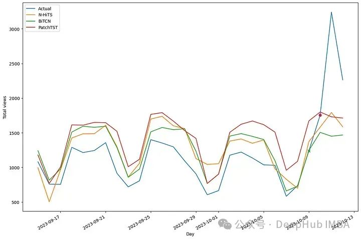
In the figure above, we can see that all models seem to have over-predicted the actual traffic. Let’s use MAE and sMAPE to see the actual comparison of the models:

from utilsforecast.losses import mae, smape
from utilsforecast.evaluation import evaluate
 evaluation = evaluate(    test_df,    metrics=[mae, smape],    models=["NHITS", "BiTCN", "PatchTST"],    target_col="y", )
 evaluation = evaluation.drop(['unique_id'], axis=1) evaluation = evaluation.set_index('metric')
 evaluation.style.highlight_min(color='blue', axis=1)

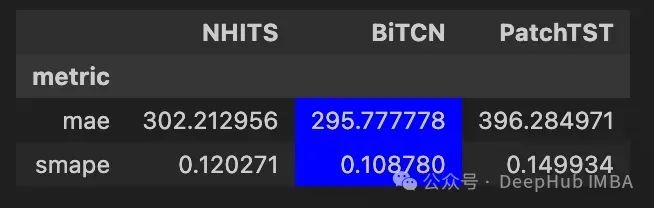
We can see that BiTCN achieved the best performance, as the MAE and sMAPE of this model are the lowest.

Although this experiment itself is not a robust benchmark for BiTCN, it demonstrates that it achieves the best results in a forecasting environment with exogenous features.

Conclusion

The BiTCN model utilizes two Temporal Convolutional Networks to encode past and future values of covariates for effective multivariate time series forecasting.

In our small experiment, BiTCN achieved the best performance, and it is interesting to see the successful application of Convolutional Neural Networks in the time series domain, as most models are based on MLP or Transformer.

Finally, the code for this article:

https://github.com/marcopeix/time-series-analysis/blob/master/bitcn_blog.ipynb

Author: Marco Peixeiro

Editor: Huang Jiyan