Applications of Deep Learning in 3D Environment Reconstruction

Click on the above“Beginner’s Visual Learning“, select to add “Starred” or “Pinned“

Important content delivered at the first time

This article is reprinted from: Computer Vision Alliance

The most classic computer vision problem is 3-D reconstruction. It can basically be divided into two paths: one is multi-view reconstruction, and the other is motion reconstruction. The former has a classic method called Multiple View Stereo (MVS), which involves multi-frame stereo matching, making it reasonable to use CNN models to solve it. Traditional MVS methods can be divided into two types: region growing and depth fusion. The 3D reconstruction and viewpoint conversion demonstrated by CMU during the Super Bowl in the U.S. was based on this path, but it was ultimately not productized (the technology has already been transferred).

The latter has become the Simultaneous Localization and Mapping (SLAM) technology in the field of robotics, which has two methods: filtering and keyframe methods. The latter has high accuracy and can use Bundle Adjustment (BA) based on sparse feature points, with famous methods such as PTAM, ORB-SLAM1/2, LSD-SLAM, KinectFusion (RGB-D data), LOAM/Velodyne SLAM (LiDAR data), etc. Structure from Motion (SFM) is based on the premise of a static background. Colleagues in computer vision prefer the term SFM, while colleagues in robotics refer to it as SLAM. SLAM focuses more on engineering solutions, while SFM contributes theoretically.

Additionally, Visual Odometry (VO) is part of SLAM, which is essentially just estimating its own motion and pose changes. VO is a concept established by David Nister, previously known for the “5-point algorithm” that computes the Essential Matrix using two frames of images.

Since CNNs have been applied in feature matching, motion estimation, and stereo matching, exploring applications in SLAM/SFM/VO/MVS has become inevitable.

DeepVO

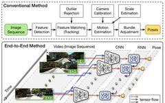
As shown in the figure, the classic VO pipeline usually includes camera calibration, feature detection, feature matching (or tracking), outlier rejection (e.g., RANSAC), motion estimation, scale estimation, and local optimization (Bundle Adjustment, BA).

DeepVO proposes an end-to-end monocular Visual Odometry (VO) framework based on deep recurrent convolutional neural networks (RCNN). Because it is trained and deployed in an end-to-end manner, it directly infers the pose from a series of raw RGB images (video) without using any modules in the traditional VO pipeline. Based on RCNN, it not only automatically learns effective feature representations for the VO problem through CNN but also implicitly models the dynamics and relationships in series using deep recurrent neural networks.

The architecture diagram of this end-to-end VO system is shown in the figure: using video segments or monocular image sequences as input; at each time step, preprocessing is performed as RGB image frames, subtracting the mean RGB value of the training set, and the image size can be adjusted to a multiple of 64; two consecutive images are stacked together to form a tensor for deep RCNN, learning how to extract motion information and estimate the pose. Specifically, the image tensor is fed into CNN to produce effective features for monocular VO, which are then learned serially through RNN. Each image pair produces pose estimates at each time step of the network. The VO system evolves over time and estimates new poses as images are acquired.

As shown in the figure, CNN has 9 convolutional layers, each followed by a ReLU activation except for Conv6, totaling 17 layers. The size of the receptive field in the network gradually decreases from 7×7 to 5×5, and then gradually to 3×3, to capture small interesting features. Zero padding is introduced to fit the configuration of the receptive field or to maintain the spatial dimensions of the tensor after convolution. The number of channels, i.e., the number of filters used for feature detection, increases to learn various features.

A deep RNN is constructed by stacking two LSTM layers, where the hidden state of one is the input of the other. In the DeepVO network, each LSTM layer has 1000 hidden states. The deep RNN outputs pose estimates at each time step based on the visual features generated from CNN. As the camera moves and acquires images, this process continues over time.

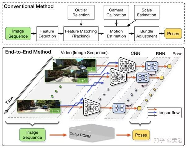
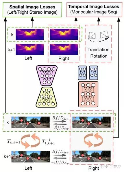
UnDeepVOUnDeepVO can estimate the 6-DoF pose of a monocular camera and the depth of its field of view using deep neural networks. There are two significant features: one is an unsupervised deep learning scheme, and the other is absolute depth recovery. When training UnDeepVO, the scale is recovered by using stereo image pairs, but during testing, continuous monocular images are used. UnDeepVO is still a monocular system. The loss function for the network training is based on spatiotemporal dense information, as shown in the figure.

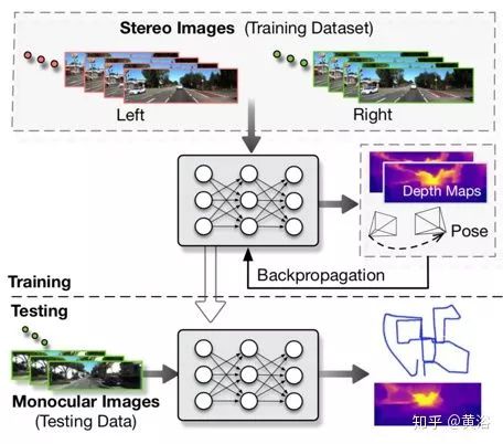
The architecture diagram of UnDeepVO is shown below. The pose estimator is based on a VGG-based CNN architecture, requiring two consecutive monocular images as input and predicting the 6-DoF transformation matrix between them. Since rotation (represented by Euler angles) is highly nonlinear and usually difficult to train compared to translation, a popular solution for supervised training is to give greater weight to the rotation estimation loss, as if normalizing. To better train rotation predictions in unsupervised learning, two sets of independent fully connected layers are used after the last convolutional layer to separate translation and rotation. This introduces a weight-normalized rotation prediction and translation prediction for better performance. The depth estimator is mainly based on an encoder-decoder architecture to generate dense depth maps. Unlike other methods, UnDeepVO directly predicts depth maps because training in this way makes the entire system easier to converge.

As shown in the figure, the loss function is defined by the spatiotemporal geometric consistency of stereo image sequences. Spatial geometric consistency indicates the epipolar constraints between corresponding points in the left and right image pairs, while temporal geometric consistency indicates the geometric projection constraints between corresponding points in two consecutive monocular images. These constraints construct the final loss function and minimize it, while UnDeepVO learns to estimate the scaled 6-DoF pose and depth maps in an end-to-end unsupervised manner. Briefly, the spatial loss function includes photometric consistency loss, disparity consistency loss, and pose consistency loss; the temporal loss function includes photometric consistency loss and 3D geometric registration loss.

VINet

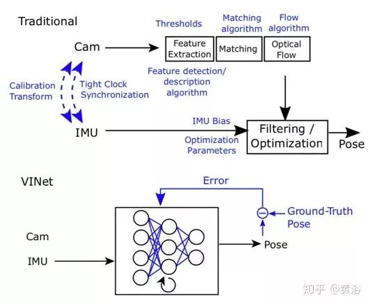
As shown in the figure, it compares traditional VIO (visual-inertial odometry) and the deep learning-based VINet method. VINet is a manifold sequence-to-sequence learning method using visual and inertial sensors for motion estimation. Its advantages include: eliminating the cumbersome manual synchronization between the camera and IMU, and no need for manual calibration; the model naturally incorporates specific domain information, significantly reducing drift.

The architecture diagram of VINet is shown below. The model includes a CNN-RNN network tailored for the VIO task. The entire network is differentiable and can be end-to-end trained for motion estimation. The input to the network is monocular RGB images and IMU data, which is a 6-dimensional vector containing the x, y, z components of acceleration and angular velocity measured by the gyroscope. The output of the network is a 7-dimensional vector – 3-dimensional translation and 4-dimensional quaternion – representing the change in pose. Essentially, it learns to map the input sequences of images and IMU data to pose.

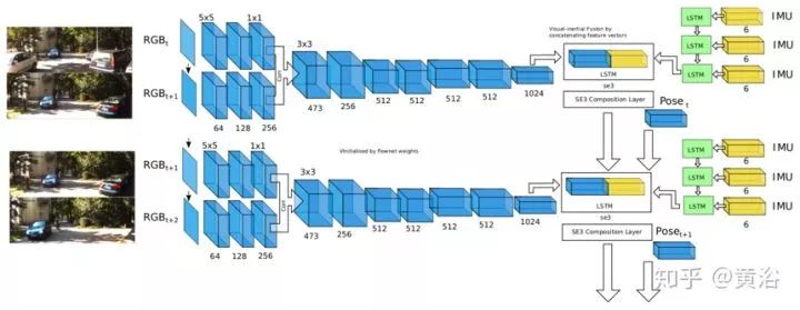
The CNN-RNN network performs the mapping from input data to the Lie algebra se(3). The exponential map converts them into the special Euclidean group SE(3), and then individual motions can be composed in SE(3) to form trajectories. In this way, the network needs to approximate the function that remains constrained over time, as the motion from frame to frame is defined by the complex dynamics of the platform during the trajectory. With the RNN model, the network can learn the complex motion dynamics of the platform while considering those sequential dependencies that are difficult to manually model. The following figure illustrates the SE(3) composition layer: a non-parametric layer that connects transformations between frames on the SE(3) group.

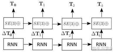
In the LSTM model, the hidden state is transferred to the next time step, but the output itself does not feedback into the input. In the case of odometry, the availability of previous states is particularly important, as the output is essentially the cumulative incremental displacement at each step. Therefore, directly connecting the pose output produced by the SE(3) composition layer serves as the input for the core LSTM of the next time step.

SfM-Net

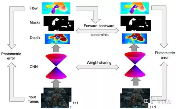
SfM-Net is a neural network for video motion estimation geometry awareness, decomposing frame pixel motion based on scene, target depth, camera motion, 3D target rotation, and translation. Given a sequence of image frames, SfM-Net predicts depth, segmentation, camera, and rigid motion, converting them into a dense frame-to-frame motion field (optical flow), allowing timely differential deformation of frames to match pixels and backpropagation. The model can be trained with varying degrees of supervision: 1) self-supervised training through reprojection photometric error (completely unsupervised), 2) self-motion (camera motion) supervised training, or 3) supervised training by depth maps (e.g., RGBD sensors).

The flowchart of SfM-Net is shown below. Given a pair of image frames as input, the model decomposes frame-to-frame pixel motion into 3D scene depth, 3D camera rotation and translation, a set of motion masks, and corresponding 3D rigid rotation and translation motion. The resulting 3D scene flow is then back-projected into 2D optical flow and deformed accordingly to match pixels from this frame to the next frame. The forward consistency check constrains the estimated depth values.

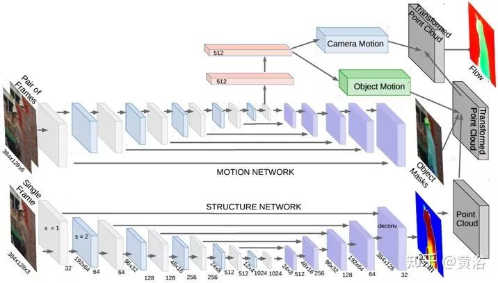
Below is the architecture diagram of SfM-Net: for each pair of consecutive frames It, It+1, a conv/deconv subnetwork predicts depth dt, while another conv/deconv subnetwork predicts a set of K segmentation masks mt; the motion mask encoder’s coarsest feature map is further decoded through fully connected layers, outputting the 3D rotation and translation for the camera and K segments; using the estimated or known camera intrinsic parameters, the predicted depth is converted into point clouds for each frame; then, based on the predicted 3D scene flow, it is transformed, composed of 3D camera motion and independent 3D mask motion; the transformed 3D depth is then projected back to the 2D next image frame, providing the corresponding 2D optical flow field; the differentiable backward deformation mapping maps the image frame It+1 to It, and the gradient can be computed based on pixel errors; the process is repeated for the reverse image frame pair It+1, It to impose “forward-backward constraints” and maintain consistency between the estimated scene motion constraints depth dt and dt+1.

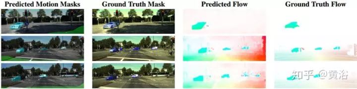
As shown in the figure, some examples of SfM-Net results. In KITTI 2015, the segmentation and optical flow of the foundational facts are compared with the motion masks and optical flow predicted by SfM-Net. The model is trained in a completely unsupervised manner.

CNN-SLAM

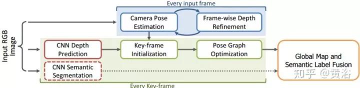
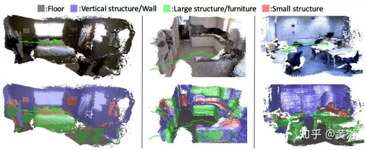
With the help of CNN’s depth map prediction method, CNN-SLAM can be used for precise and dense monocular image reconstruction. The dense depth maps predicted by CNN and the depth results obtained directly from monocular SLAM are fused together. In low-texture areas where monocular SLAM is close to failure, its fusion scheme gives priority to depth prediction, and vice versa. Depth prediction can estimate the absolute scale of the reconstruction, overcoming a major limitation of monocular SLAM. Finally, the semantic labels obtained from a single frame and the dense SLAM fusion can yield semantically coherent single-view scene reconstruction results.

As shown in the figure, the architecture diagram of CNN-SLAM is presented. CNN-SLAM adopts a keyframe-based SLAM paradigm, particularly using a direct semi-dense method as a benchmark. This method collects different visual frames as keyframes, whose poses are globally corrected through pose-graph optimization methods. Meanwhile, pose estimation for each input frame is achieved by estimating the transformation between the frame and its nearest keyframe.

Below are some results: office scene (left) and two kitchen scenes from the NYU Depth V2 dataset (middle, right), with the first row showing reconstructions and the second row showing semantic labels.

PoseNet

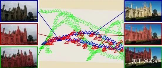
PoseNet is a real-time monocular 6-DOF relocalization system. It trains a CNN model to regress 6-DOF camera poses from RGB images in an end-to-end manner without the need for additional engineering or graphical optimization. The algorithm can run in real-time both indoors and outdoors, with 5ms per frame. Through an effective 23-layer deep convolutional network, PoseNet achieves regression in the image plane, robust to scenes with poor lighting, motion blur, and varying intrinsic parameters (where SIFT calibration fails). The generated pose features can be generalized to other scenes, allowing pose parameters to be regressed with only a few dozen training examples.

PoseNet uses GoogLeNet as the basis for the pose regression network; it replaces all three softmax classifiers with affine regressors; removes the softmax layer and modifies each final fully connected layer output to represent the 7-dimensional pose vector of 3D position (3) and orientation quaternion (4); inserts another fully connected layer before the final regressor with a feature size of 2048; during testing, the quaternion orientation vector is normalized to unit length.

As shown in the figure, the results of PoseNet are displayed. Green represents training examples, blue represents testing examples, and red shows pose predictions.

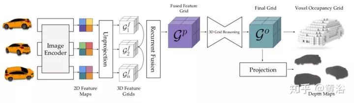
It should be noted that pose regression employs the following target loss function for training through stochastic gradient descent:

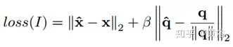
Where x is the position vector, q is the quaternion vector, and β is the chosen scale factor to keep the expected values of position and orientation errors approximately equal.

VidLoc

VidLoc is a recursive convolution model for video segment 6-DoF localization. Even considering only short sequences (20 frames), it can smooth the pose estimates and significantly reduce localization errors.

As shown in the figure, the architecture model of VidLoc is presented. The goal of the CNN part is to extract relevant features from the input images that can be used to predict the global pose of the image. The CNN consists of stacked convolutional and pooling layers that operate on the input images. Here, it mainly processes multiple images in temporal order, using the GoogleNet architecture of VidLoc CNN, which actually only uses the convolutional and pooling layers of GoogleNet and removes all fully connected layers.

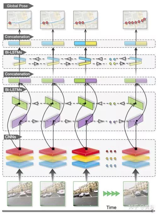
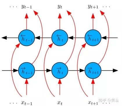
When inputting a continuous stream of images over time, utilizing temporal regularities can yield a wealth of pose information. For instance, adjacent images often contain views of the same target, which can enhance confidence at specific locations, and there are strict constraints on motion between frames. To capture these dynamic correlations, the network employs an LSTM model. LSTM extends the standard RNN, capable of learning long-term temporal dependencies, achieved through forget gates, input and output reset gates, and memory units. The input to LSTM is the output from CNN, consisting of a series of feature vectors xt. LSTM maps the input sequence to the output sequence, with the output sequence parameterized as a 7-dimensional vector of global pose yt, including translation vector and orientation quaternion. To fully utilize temporal continuity, the LSTM model here adopts a bidirectional structure, as shown in the figure.

To simulate the uncertainty of pose estimation, a mixture density networks method is employed. This approach replaces the Gaussian model with a mixture model, allowing for the modeling of multi-modal posterior output distributions.

NetVLAD

The large-scale visual-based location recognition problem requires rapid and accurate identification of the location of a given query photo. NetVLAD is a layer in a CNN architecture that helps the entire architecture be used for location recognition in an end-to-end manner. Its main component is a universal “Vector of Locally Aggregated Descriptors” (VLAD) layer, inspired by the VLAD pooling method for feature descriptors in image retrieval. This layer can easily be inserted into any CNN architecture and can be trained through backpropagation (BP). Based on a defined weakly supervised ranking loss, it can be trained using images of the same location downloaded from Google Street View Time Machine to learn the architecture parameters in an end-to-end manner.

As shown in the figure, the CNN structure with the NetVLAD layer is presented. This layer implements the “VLAD kernel” aggregation with standard CNN layers (convolution, softmax, L2 normalization) and an easily implementable aggregation layer NetVLAD that connects in a directed acyclic graph (DCG).

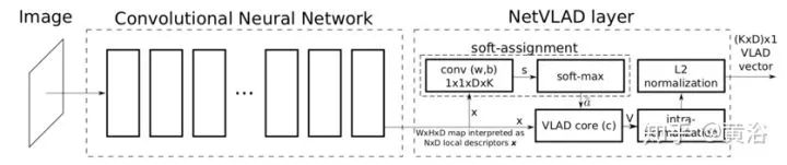
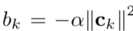
Given N D-dimensional local image feature descriptors {xi} as input, K clustering centers (“visual words”) {ck} serve as VLAD parameters, outputting the VLAD image representation V as a K×D dimensional matrix. This matrix can be converted into a vector, normalized, and used as the image representation. The (j,k) element of V is calculated as follows:

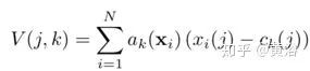
Where xi(j) and ck(j) are the j-th dimension of the i-th feature descriptor and the k-th clustering center, respectively. ak(xi) records the membership of descriptor xi to the k-th visual word, which is 1 if cluster ck is the closest cluster to explain xi, otherwise 0.

The discontinuity of VLAD arises from the hard assignment ak(xi) of descriptors xi to clustering centers ck. To make it differentiable, it is replaced with a soft assignment of descriptors to multiple clusters, i.e.

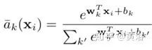
By expanding the square term of the above equation, it is easy to see that the exp() term cancels out between the numerator and denominator, leading to the following soft assignment:

Where the vector wk and scalar bk

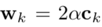
Thus, the final “VLAD kernel” aggregation formula becomes

Where {wk}, {bk}, and {ck} are the trainable parameters for each cluster k.

In VLAD encoding, the contribution of two feature descriptors belonging to the same cluster but from different images is measured by the scalar product of the residual vectors between the two images, where the residual vector is the difference between the descriptor and the clustering anchor point. The anchor point ck can be interpreted as the new coordinate system origin for the specific cluster k. In standard VLAD, the anchor points are chosen as clustering centers (×) to ensure that the residuals in the database are evenly distributed. However, as shown in the figure, in a supervised learning setup, two descriptors from mismatched images can learn better anchors, making the new residual vectors have a small scalar product.

Learned Stereo Machine

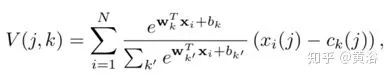
The Learning Stereo Machine (LSM) is a deep learning system for multi-view stereo vision proposed by UC Berkeley. Compared to other recent learning-based 3D reconstruction methods, it utilizes the underlying 3D geometric relationships of the problem by performing feature projection and back-projection along the viewing rays. By defining these operations in a differentiable manner, it allows for end-to-end learning of the system for measuring 3D reconstruction tasks. This end-to-end learning can jointly reason about prior knowledge of shapes while satisfying geometric constraints, enabling reconstruction with fewer images (even a single image) and completing unseen surfaces.

As shown in the figure, an overview of LSM is presented: one or more views and camera poses as input; the images are processed through a feature encoder, and then projected into the 3D world coordinate system using differentiable back-projection operations.

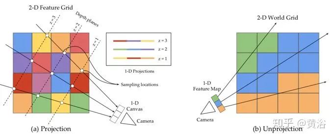
As shown, a schematic diagram of projection and back-projection between a 1D image and a 2D grid is provided. (a) The projection operation samples values at equal intervals z along the rays into the 1D image. The sampled features in the z-plane are stacked into channels to form the projected feature map. (b) The back-projection operation retrieves features from the feature map (1-D) and places them in the corresponding grid blocks intersecting along the rays.

Then, these grids G are recursively matched to generate a fused grid Gp, where a gated recurrent unit (GRU) model is employed. Finally, LSM can produce two outputs – a voxel occupancy grid (voxel LSM) decoded from Go or depth maps for each view decoded after the projection operation (depth LSM).

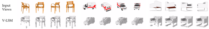
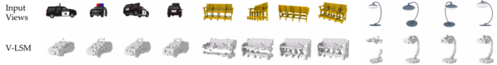
The following figures show some results of V-LSM,

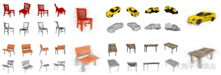
As shown, some examples of D-LSM are provided.

DeepMVS

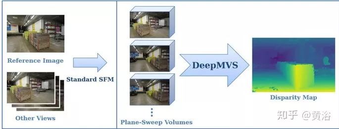
DeepMVS is a deep convolutional neural network (ConvNet) for multi-view stereo (MVS) reconstruction. It takes an arbitrary number of images from various poses as input, first producing a set of plane-sweep volumes and using the DeepMVS network to predict high-quality disparity maps. Its key features are (1) pre-training on photorealistic synthetic datasets; (2) an effective way to aggregate information on a set of unordered images; (3) integrating multi-layer feature activation functions in the pre-trained VGG-19 network. DeepMVS’s effectiveness has been validated using the ETH3D benchmark.

The algorithm process is divided into four steps. First, the input image sequence is preprocessed, then plane-sweep volumes are generated. Next, the network estimates the disparity maps of the plane-sweep volumes, and finally refines the results, as shown in the figure.

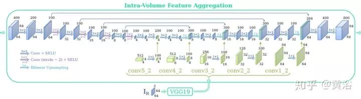
The following two figures show the architecture of DeepMVS with hyperparameters. The entire network is divided into three parts: 1) patch matching network, 2) intra-volume feature aggregation network, and 3) inter-volume feature aggregation network. All convolutional layers in the network, except for the last layer, are followed by a Scaled Exponential Linear Unit (SELU) layer.

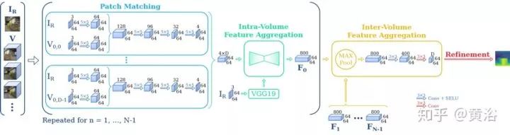
To further improve performance, a fully connected conditional random field (DenseCRF) is applied to the disparity prediction results.

MVSNet

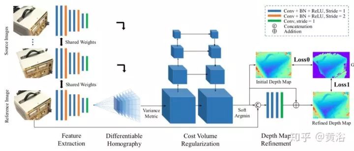
Given a reference image I1 and a set of its adjacent images {Ii} Ni = 2, MVSNet proposes an end-to-end deep neural network to infer the reference depth map D. In its network, depth image features { Fi} Ni = 1 are first extracted from the input images through a 2D network. Then, the 2D image features are deformed into the reference camera coordinate system through a differentiable homography transformation, constructing feature volumes {Vi} Ni = 1 in 3D space. To handle arbitrary N view images as input, a variance-based cost measure maps the N feature volumes to a cost volume C. Similar to other stereo vision and MVS algorithms, MVSNet uses multi-scale 3D CNN to regularize the cost volume and regresses the reference depth map D through soft argmin operation. At the end of MVSNet, a refinement network is applied to further enhance the performance of the predicted depth map. Since the depth image features {Fi} Ni = 1 are downscaled during feature extraction, the output depth map size is 1/4 of the original image size in each dimension.

MVSNet demonstrates state-of-the-art performance on the DTU dataset and the intermediate set of the Tanks and Temples dataset, which contains scenes with “look-from-outside” camera trajectories and small depth ranges. However, using a 16 GB memory Tesla P100 GPU card, MVSNet can only handle a maximum reconstruction scale of H×W×D = 1600×1184×256 and will fail in larger scenes, such as the advanced collection of Tanks and Temples.

As shown in the figure, the design diagram of the MVSNet network is presented. Input images generate cost volumes through a 2D feature extraction network and differentiable homography deformation. The final depth map output is regressed from the regularized probability volume and refined with the reference image.

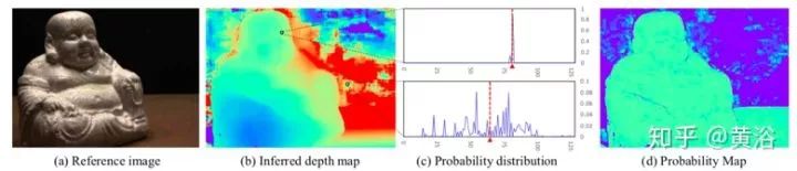
The following figure shows the inferred depth map, probability distribution, and probability graph. (a) A reference image from the DTU dataset; (b) the inferred depth map; (c) the probability distributions of inlier pixels (top) and outlier pixels (bottom), where the x-axis is the depth hypothesis index, y-axis is probability, and the red line is the soft argmin result; (d) probability graph.

•Recurrent MVSNet

A major limitation of MVS methods is scalability: the memory-intensive cost volume regularization makes learned MVS difficult to apply to high-resolution scenes. Recurrent MVSNet is a scalable multi-view stereo vision framework based on recurrent neural networks. The recurrent multi-view stereo vision network (R-MVSNet) does not regularize the entire 3D cost volume at once, but serially regularizes the 2D cost map along the depth value direction through a gated recurrent unit (GRU) network. This greatly reduces memory consumption and enables high-resolution reconstruction.

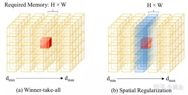
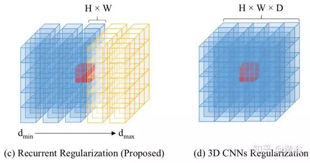
The following figure compares the strategies of different regularization schemes. The alternative to one-time global regularization of the cost volume C is to process the cost volume serially along the depth direction. The simplest sequential approach is the winner-takes-all (WTA) plane-sweeping stereo vision method, which roughly replaces pixel depth values with better values, thus being susceptible to noise (as shown in figure (a)). To address this, the cost aggregation method filters the matching cost volume C(d) at different depths (as shown in figure (b)) to collect spatial contextual information for each cost estimate. Following the idea of serial processing, a stronger recursive regularization scheme based on convolutional GRU is employed here. This method can collect spatial and unidirectional contextual information in the depth direction (as shown in figure (c)), achieving nearly the same regularization results compared to full spatial 3D CNN (as shown in figure (d)), but with more efficient runtime memory.

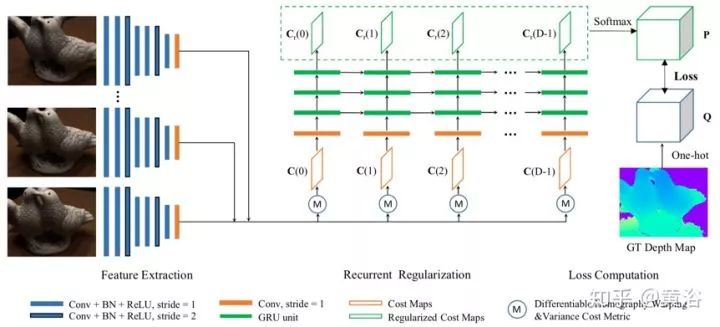
The following figure introduces the framework of R-MVSNet. It extracts depth image features from the input images and then deforms them to the reference camera coordinate system along the forward parallel plane. The cost map is computed at different depths and processed serially by the convolutional GRU. The network is trained as a classification problem with cross-entropy loss.

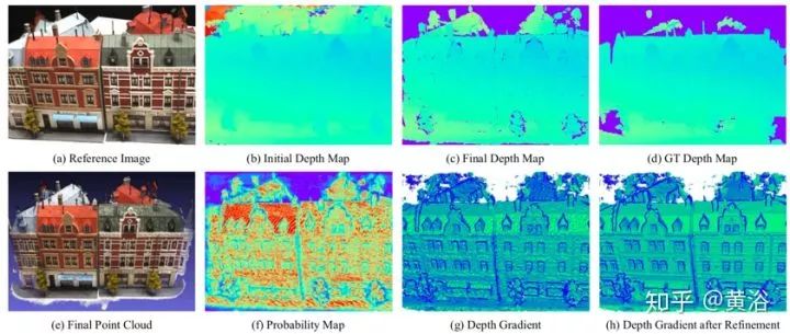
As shown in the figure, the intuitive diagram of the reconstruction pipeline of R-MVSNet is presented: (a) DTU images; (b) initial depth maps from the network; (c) final depth map estimates; (d) ground truth depth maps; (e) output point clouds; (f) probability estimation maps for depth map filtering; (g) gradient maps of the initial depth maps; (h) refined gradient maps.

References

• 1. Kendall A, Grimes M, Cipolla R. “PoseNet: A convolutional network for real-time 6-DoF camera relocalization”, IEEE ICCV. 2015

• 2. Li X, Belaroussi R. “Semi-Dense 3D Semantic Mapping from Monocular SLAM”. arXiv 1611.04144, 2016.

• 3. J McCormac et al. “SemanticFusion: Dense 3D semantic mapping with convolutional neural networks”. arXiv 1609.05130, 2016

• 4. R Arandjelovic et al. “NetVLAD: CNN architecture for weakly supervised place recognition”, CVPR 2016

• 5. B Ummenhofer et al., “DeMoN: Depth and Motion Network for Learning Monocular Stereo”, CVPR 2017

• 6. R Li et al. “UnDeepVO: Monocular Visual Odometry through Unsupervised Deep Learning”. arXiv 1709.06841, 2017.

• 7. S Wang et al.,“DeepVO: Towards End-to-End Visual Odometry with Deep Recurrent Convolutional Neural Networks”, arXiv 1709.08429, 2017

• 8. R Clark et al. “VidLoc: 6-DoF video-clip relocalization”. arXiv 1702.06521，2017

• 9. R Clark et al. “VINet: Visual-Inertial Odometry as a Sequence-to-Sequence Learning Problem.” AAAI. 2017

• 10. D DeTone, T Malisiewicz, A Rabinovich. “Toward Geometric Deep SLAM”. arXiv 1707.07410, 2017.

• 11. S Vijayanarasimhan et al.,“SfM-Net: Learning of Structure and Motion from Video”, arXiv 1704.07804, 2017

• 12. K Tateno K et al. “CNN-SLAM: Real-time dense monocular SLAM with learned depth prediction”. arXiv 1704.03489, 2017.

• 13. J Zhang et al. “Neural SLAM : Learning to Explore with External Memory”，arXiv 1706.09520， 2017

• 14. Wu J, Ma L, Hu X. “Delving deeper into convolutional neural networks for camera relocalization”，IEEE ICRA, 2017

• 15. A Kar, C Haene, J Malik, “Learned Stereo Machine”, NIPS, 2017

• 16. P Huang et al.,“DeepMVS: Learning Multi-view Stereopsis”, CVPR 2018

• 17. Y. Yao et al., “MVSNet: Depth inference for unstructured multi-view stereo”. ECCV，2018.

• 18. Y Yao et al.,“Recurrent MVSNet for High-resolution Multi-view Stereo Depth Inference”, CVPR 2019

• 19. G Zhai et al.,“PoseConvGRU: A Monocular Approach for Visual Ego-motion Estimation by Learning”, arXiv 1906.08095, 2019

• 20. X Han, H Laga, M Bennamoun,“Image-based 3D Object Reconstruction: State-of-the-Art and Trends in the Deep Learning Era”, arXiv 1906.06543, 2019

Good news!
The Beginner's Visual Learning Knowledge Planet
is now open to the outside world👇👇👇





Download 1: OpenCV-Contrib Extension Module Chinese Version Tutorial
Reply "Extension Module Chinese Tutorial" in the "Beginner's Visual Learning" public account backend to download the first OpenCV extension module tutorial in Chinese, covering more than twenty chapters including extension module installation, SFM algorithm, stereo vision, target tracking, biological vision, super-resolution processing, etc.

Download 2: Python Visual Practical Project 52 Lectures
Reply "Python Visual Practical Project" in the "Beginner's Visual Learning" public account backend to download 31 visual practical projects including image segmentation, mask detection, lane detection, vehicle counting, adding eyeliner, license plate recognition, character recognition, emotion detection, text content extraction, facial recognition, etc., to help quickly learn computer vision.

Download 3: OpenCV Practical Project 20 Lectures
Reply "OpenCV Practical Project 20 Lectures" in the "Beginner's Visual Learning" public account backend to download 20 practical projects based on OpenCV, achieving advanced learning of OpenCV.

Group Chat

Welcome to join the public account reader group to communicate with peers. There are currently WeChat groups for SLAM, 3D vision, sensors, autonomous driving, computational photography, detection, segmentation, recognition, medical imaging, GAN, algorithm competitions, etc. (will gradually be subdivided in the future). Please scan the WeChat number below to join the group, and note: "Nickname + School/Company + Research Direction", for example: "Zhang San + Shanghai Jiao Tong University + Visual SLAM". Please follow the format; otherwise, you will not be approved. After successful addition, you will be invited to enter the relevant WeChat group based on research direction. No advertisements should be sent in the group; otherwise, you will be removed from the group. Thank you for your understanding~