
Source: AI Technology Review, DataPi THU


This article is about 7100 words long and is recommended for a 13-minute read.
It summarizes the historical origins of several foundational algorithms in the field of machine learning.
 Recently, Andrew Ng updated a blog post on his founded AI Weekly, “The Batch”, summarizing the historical origins of several foundational algorithms in the field of machine learning.At the beginning of the article, Andrew Ng recalls a choice he had to make during his research journey:Many years ago, during a project, he had to choose between neural networks and decision tree learning algorithms when selecting an algorithm. Considering the computational budget, he ultimately chose neural networks and abandoned the boosted decision trees for a long time.This was a wrong decision. “Fortunately, my team quickly corrected my choice, and the project succeeded,” Andrew Ng said.He lamented that continuously learning and updating foundational knowledge is very important. Like other technical fields, as the number of researchers and research results increases, the field of machine learning is also constantly evolving. However, some foundational algorithms and core concepts have stood the test of time:
- Algorithms: Linear and logistic regression, decision trees, etc.
- Concepts: Regularization, optimizing loss functions, bias/variance, etc.
In Andrew Ng’s view, these algorithms and concepts are the core ideas behind many machine learning models, including house price predictors, text-image generators (like DALL·E), and more.In this latest article, Andrew Ng and his team researched the origins, uses, evolutions, and provided detailed explanations of six foundational algorithms.The six algorithms are: linear regression, logistic regression, gradient descent, neural networks, decision trees, and k-means clustering algorithms.1. Linear Regression: Straight & NarrowLinear regression is a key statistical method in machine learning, but it is not without its challenges. It was proposed by two outstanding mathematicians, and even after 200 years, the problem remains unsolved. The long-standing controversy not only proves the remarkable practicality of the algorithm but also demonstrates its inherent simplicity.So whose algorithm is linear regression?In 1805, French mathematician Adrien-Marie Legendre published a method for fitting a line to a set of points while attempting to predict the position of a comet (celestial navigation was the most valuable scientific direction in global commerce at the time, much like today’s AI).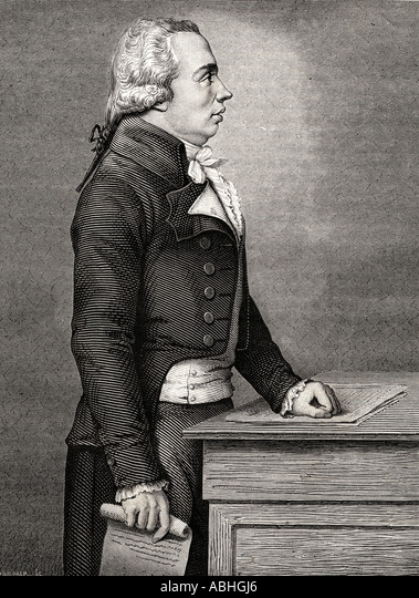 Caption: Portrait of Adrien-Marie LegendreFour years later, 24-year-old German prodigy Carl Friedrich Gauss insisted he had been using it since 1795 but thought it was too trivial to write about. Gauss’s claim prompted Legendre to anonymously publish a paper stating, “A very famous geometer has unhesitatingly adopted this method.”
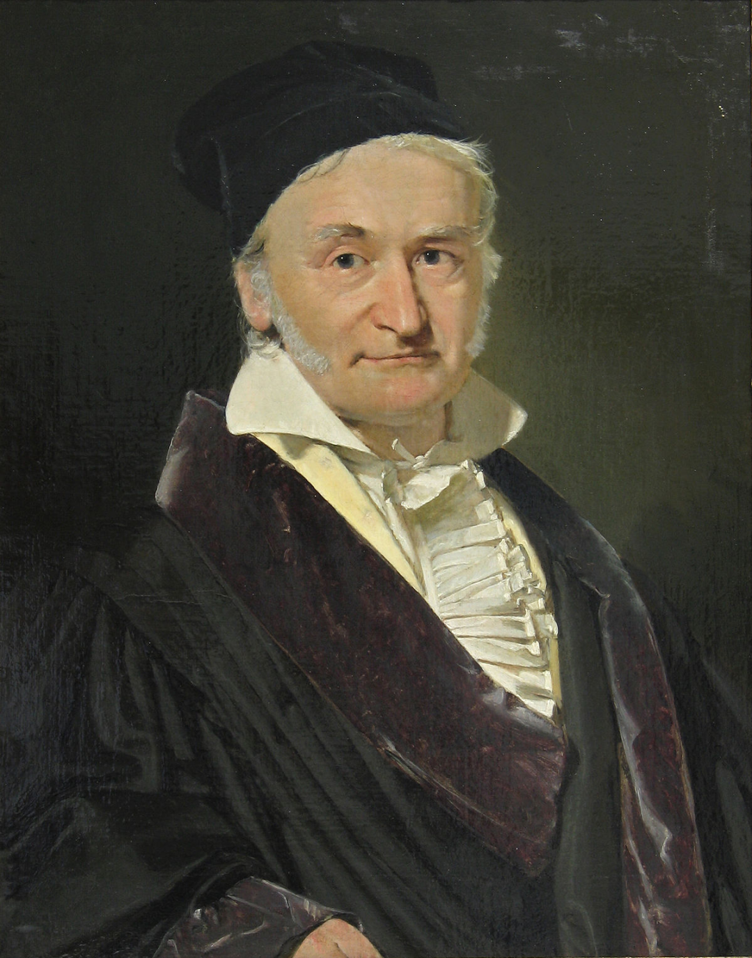 Caption: Carl Friedrich GaussSlope and Bias:Linear regression is useful when the relationship between the result and the variables affecting it follows a straight line. For example, a car’s fuel consumption has a linear relationship with its weight.
- The relationship between a car’s fuel consumption y and its weight x depends on the slope w (the increase in fuel consumption with weight) and the bias term b (fuel consumption when weight is zero): y=w*x+b.
- During training, given the weight of the car, the algorithm predicts the expected fuel consumption. It compares the expected and actual fuel consumption. Then, it minimizes the squared difference, typically through ordinary least squares techniques, refining the values of w and b.
- Considering the drag of the car can generate more accurate predictions. Additional variables extend the line into a plane. In this way, linear regression can accommodate any number of variables/dimensions.
Two Steps to Popularity:This algorithm immediately helped navigators track stars and later helped biologists (especially Francis Galton, a cousin of Charles Darwin) identify heritable traits in plants and animals. These two deep developments unleashed the broad potential of linear regression. In 1922, British statisticians Ronald Fisher and Karl Pearson demonstrated how linear regression fits into the general statistical framework of correlation and distribution, making it useful across all sciences. Moreover, nearly a century later, the advent of computers provided the data and processing power to utilize it to a greater extent.Dealing with Ambiguity:Of course, data is never perfectly measured, and some variables are more important than others. These real-life facts inspired more complex variants. For example, linear regression with regularization (also known as “ridge regression”) encourages linear regression models not to rely too heavily on any one variable, or more precisely, to evenly rely on the most important variables. For simplicity, another form of regularization (L1 instead of L2) produces lasso (compressed estimates), encouraging as many coefficients as possible to be zero. In other words, it learns to select variables with high predictive power and ignore the rest. Elastic net combines these two types of regularization. It is useful when the data is sparse or features appear correlated.In Each Neuron:Now, the simple version remains very useful. The most common type of neuron in neural networks is the linear regression model, followed by non-linear activation functions, making linear regression a fundamental component of deep learning.2. Logistic Regression: Following the CurveThere was a time when logistic regression was only used to classify one thing: if you drank a bottle of poison, would you be labeled as “alive” or “dead”? Times have changed, and today, not only do emergency services provide better answers to this question, but logistic regression has also become central to deep learning.Poison Control:The logistic function can be traced back to the 1830s when Belgian statistician P.F. Verhulst invented it to describe population dynamics: over time, the initial explosion of exponential growth flattens as it consumes available resources, resulting in a characteristic logistic curve. More than a century later, American statistician E.B. Wilson and his student Jane Worcester designed logistic regression to calculate how much of a given harmful substance is lethal.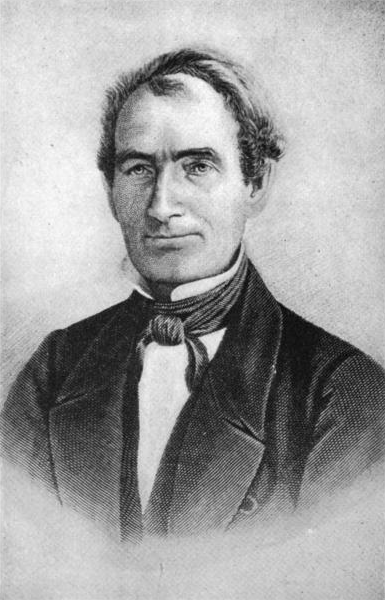 Caption: P.F. VerhulstFitting the Function:Logistic regression fits the logistic function to a dataset to predict the probability of a specific outcome (e.g., ingestion of strychnine) occurring (e.g., premature death).
- The training level adjusts the center position of the curve, and the vertical adjustment maximizes the function’s output error with the data.
- Adjusting the center to the right or left means that more or less poison is needed to kill an average person. A steep slope means certainty: most people survive before the midpoint; beyond half, “it’s just goodbye” (meaning death). A gentle slope is more forgiving: below the middle of the curve, more than half survive; further up, less than half will survive.
- Setting a threshold between one outcome and another, such as 0.5, turns the curve into a classifier. Simply input the dose into the model, and you will know whether to plan a party or a funeral.
More Outcomes:Verhulst’s work discovered the probability of binary outcomes, ignoring further possibilities, such as which side of the afterlife a poisoned victim might enter. His successors expanded the algorithm:
- In the late 1960s, British statistician David Cox and Dutch statistician Henri Theil worked independently on logistic regression for cases with more than two possible outcomes.
- Further work produced ordered logistic regression, where the outcomes are ordered values.
- To handle sparse or high-dimensional data, logistic regression can utilize the same regularization techniques as linear regression.
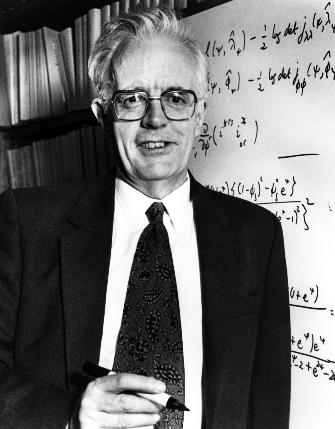 Caption: David CoxVersatile Curve: The logistic function describes a wide range of phenomena quite accurately, so logistic regression provides useful baseline predictions in many scenarios. In medicine, it can estimate mortality and disease risk. In political science, it predicts election winners and losers. In economics, it predicts business prospects. More importantly, it drives part of the neurons in various neural networks (where non-linearity is the Sigmoid function).3. Gradient Descent: Everything Goes DownhillImagine hiking on a mountain after dusk, finding nothing below your feet. And your phone battery is dead, so you can’t use the GPS app to find your way home. You might find the fastest path down using gradient descent. Be careful not to walk off a cliff.The Sun and the Carpet:Gradient descent is more advantageous than descending through steep terrain. In 1847, French mathematician Augustin-Louis Cauchy invented an algorithm for approximating stellar orbits. Sixty years later, his compatriot Jacques Hadamard independently developed it to describe the deformation of thin and flexible objects (like carpets), which might make hiking down easier. However, in machine learning, its most common use is to find the lowest point of the loss function of learning algorithms.
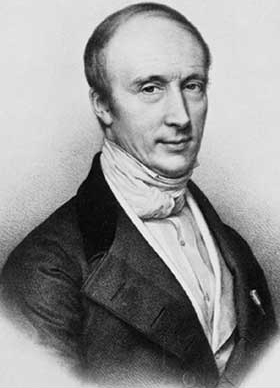 Caption: Augustin-Louis CauchyClimbing Down:A trained neural network provides a function that calculates the desired output given an input. One way to train the network is by iteratively calculating the difference between the actual output and the expected output, then changing the network’s parameter values to reduce that difference, thereby minimizing the loss or error in the output. Gradient descent reduces the difference, minimizing the function that calculates the loss. The network’s parameter values are equivalent to a position on the terrain, and the loss is the current height. As you descend, you can improve the network’s ability to compute closer to the desired output. Visibility is limited since, in typical supervised learning scenarios, the algorithm relies solely on the parameter values of the network and the gradient or slope of the loss function—that is, your position on the mountain and the slope beneath your feet.
- The basic method is to move in the steepest direction down the terrain. The trick is to calibrate your step size. If the step size is too small, it will take a long time to make progress; if the step size is too large, you might jump into unknown territory, possibly uphill instead of downhill.
- Given your current position, the algorithm estimates the fastest descent direction by calculating the gradient of the loss function. If the gradient points uphill, the algorithm moves in the opposite direction by subtracting a small portion of the gradient. A fraction called the learning rate α determines the step size before measuring the gradient again.
- Repeat these steps, hoping to reach a valley. Congratulations!
Stuck in the Valley: Too bad your phone is dead because the algorithm might not have pushed you to the bottom of a convex mountain. You might get stuck in a non-convex landscape consisting of multiple valleys (local minima), peaks (local maxima), saddle points, and plateaus. In fact, tasks like image recognition, text generation, and speech recognition are non-convex, and many variants of gradient descent have emerged to handle these situations. For example, the algorithm might have momentum to help it magnify small rises and falls, making it more likely to reach the bottom. Researchers have designed so many variants that it seems the number of optimizers is as numerous as local minima. Fortunately, local minima and global minima often roughly equal.Optimal Optimizer: Gradient descent is the clear choice for finding the minimum of any function. In cases where an exact solution can be computed directly—such as in linear regression tasks with many variables—it can approximate a value and is often faster and cheaper. But it does indeed work in complex nonlinear tasks. With gradient descent and a spirit of adventure, you might make it out of the mountains in time for dinner.4. Neural Networks: Finding FunctionsLet’s clarify this issue first: The brain is not a set of graphic processing units; if it were, the software it runs would be far more complex than a typical artificial neural network. Neural networks draw inspiration from the structure of the brain: layers of interconnected neurons, each neuron computes its output based on the states of its neighbors, resulting in a series of activities that form an idea—or recognize a picture of a cat.From Biological to Artificial:The idea that the brain learns through interactions between neurons dates back to 1873, but it wasn’t until 1943 that American neuroscientists Warren McCulloch and Walter Pitts established a biological neural network model using simple mathematical rules. In 1958, American psychologist Frank Rosenblatt developed the Perceptron—a single-layer visual network implemented on a punch card machine designed to create a hardware version for the U.S. Navy.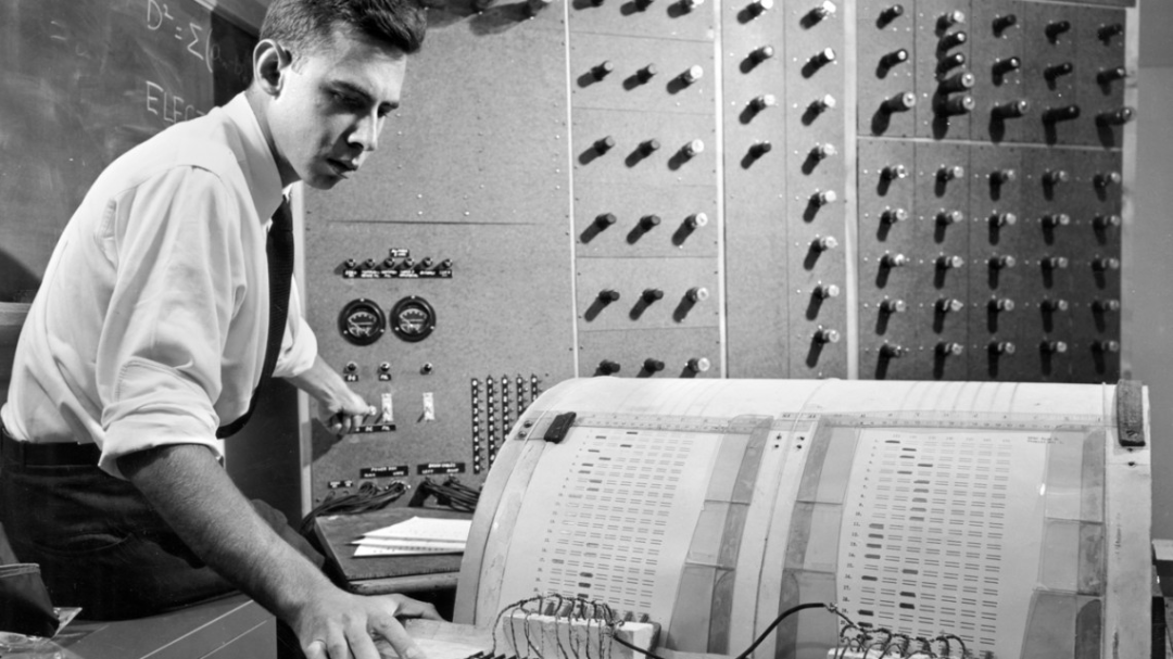 Caption: Frank RosenblattThe Bigger the Better:Rosenblatt’s invention could only recognize single-line classifications. Later, Ukrainian mathematicians Alexey Ivakhnenko and Valentin Lapa overcame this limitation by stacking networks of neurons in arbitrary layers. In 1985, French computer scientists Yann LeCun, David Parker, and American psychologist David Rumelhart and their colleagues described effectively training such networks using backpropagation. In the first decade of the new millennium, researchers, including Kumar Chellapilla, Dave Steinkraus, and Rajat Raina (who collaborated with Andrew Ng), further advanced neural networks by utilizing graphic processing units, enabling increasingly larger networks to learn from the massive data generated from the internet.Suitable for Every Task:The principle behind neural networks is simple: there is a function that can execute any task. A neural network constitutes a trainable function by combining multiple simple functions, each executed by a single neuron. The function of a neuron is determined by adjustable parameters called “weights.” Given these weights and random values for input examples and their desired outputs, the weights can be repeatedly modified until the trainable function can accomplish the task at hand.
- A neuron can accept various inputs (e.g., numbers representing pixels or words, or outputs from the previous layer), multiply them by weights, sum the products, and derive the total from a nonlinear function or activation function chosen by the developer. During this process, it considers whether it is linear regression plus an activation function.
- Training modifies weights. For each example input, the network calculates an output and compares it with the expected output. Backpropagation can change the weights via gradient descent to reduce the difference between the actual output and the expected output. When enough (good) examples repeat this process enough times, the network can learn to perform the task.
The Black Box:While a well-trained network can accomplish its task if lucky, ultimately reading a function can often be very complex—containing thousands of variables and nested activation functions—making it challenging to explain how the network successfully completes its task. Moreover, a trained network is only as good as the data it learned from. For example, if the dataset is biased, the network’s output will also be biased. If it only contains high-resolution images of cats, its response to low-resolution images remains unknown.A common sense: When reporting on the Perceptron invented by Rosenblatt in 1958, The New York Times paved the way for AI hype, mentioning that “the U.S. Navy expects to have a prototype of an electronic computer that can walk, talk, see, write, self-replicate, and be aware of its existence.” Although the Perceptron did not meet this requirement at the time, it produced many impressive models: convolutional neural networks for images; recurrent neural networks for text; and transformers for images, text, speech, video, protein structure, etc. They have accomplished astonishing feats, such as outperforming human levels in games like Go and approaching human levels in practical tasks like diagnosing X-ray images. However, they still struggle with common sense and logical reasoning issues.5. Decision Trees: From Root to LeafWhat kind of “beast” was Aristotle? This philosopher’s follower, Porphyry, who lived in Syria during the third century, devised a logical way to answer this question. He combined Aristotle’s proposed “categories of existence” from general to specific, classifying Aristotle step by step: Aristotle’s existence is material rather than conceptual or spiritual; his body is alive rather than lifeless; his mind is rational rather than irrational. Thus, his classification is human. Medieval logic teachers depicted this sequence as a vertical flowchart: an early decision tree.Numerical Differences:Fast forward to 1963, when University of Michigan sociologist John Sonquist and economist James Morgan first implemented decision trees in computers while grouping survey respondents. With the emergence of automated training algorithm software, this work became common, and various machine learning libraries, including scikit-learn, now use decision trees. This code was developed over ten years by four statisticians from Stanford University and the University of California, Berkeley. Today, writing decision trees from scratch has become a homework assignment in “Machine Learning 101.”Roots in the Air:Decision trees can perform classification or regression. They grow downwards from root to canopy, classifying input examples of a decision hierarchy into two (or more). Consider the subject of German physician and anthropologist Johann Blumenbach: around 1776, he was the first to distinguish monkeys from apes (excluding humans), whereas monkeys and apes had previously been classified together. This classification depended on various criteria, such as whether they had tails, narrow or broad chests, whether they were upright or crouched, and their level of intelligence. Using a trained decision tree to label these animals, one considers each criterion one by one, ultimately separating the two groups of animals.
- The tree starts from a root node that can be viewed as containing all cases—a database of chimpanzees, gorillas, and orangutans, as well as macaques, baboons, and tamarins. The root offers choices between two child nodes, whether to exhibit a specific characteristic, leading to two child nodes containing examples with and without that characteristic. This process continues with any number of leaf nodes, each containing most or all examples belonging to a category.
- To grow, the tree must find root decisions. To make a choice, all features and their values must be considered—hind limbs, barrel-shaped chest, etc.—and choose the feature that maximizes the purity of the split. “Best purity” is defined as a category example entering a specific child node 100% of the time and not entering another node. Branching rarely achieves 100% purity after just one decision and is unlikely to ever reach that. As this process continues, one level of child nodes after another is produced until the purity does not increase significantly by considering more features. At this point, the tree has been fully trained.
- During inference, a new example traverses the decision tree from top to bottom, completing evaluations of different decisions at each level. It receives the data label contained in the leaf node it ends up in.
Entering the Top 10:Given Blumenbach’s conclusion (later overturned by Charles Darwin) that the distinction between humans and apes lies in the broad pelvis, hands, and tightly packed teeth, what if we wanted to expand the decision tree to classify humans as well? Australian computer scientist John Ross Quinlan achieved this possibility in 1986 through ID3, which extended decision trees to support non-binary outcomes. In 2008, a refinement algorithm named C4.5 ranked high on a list of the top ten data mining algorithms curated at the IEEE International Conference on Data Mining. In a world rife with innovation, this is persistence.Peeling Back the Leaves:Decision trees do have some drawbacks. They can easily overfit data by adding multiple levels of hierarchy, such that leaf nodes only include one example. Worse still, they can easily exhibit the butterfly effect: change one example, and the resulting tree can be significantly different.Walking into the Forest:American statistician Leo Breiman and New Zealand statistician Adele Cutler turned this feature into an advantage by developing the random forest in 2001—a collection of decision trees, each handling different overlapping sample selections and voting on the final outcome. Random forests and their cousin XGBoost are less prone to overfitting, helping make them one of the most popular machine learning algorithms. It’s like having Aristotle, Porphyry, Blumenbach, Darwin, Jane Goodall, Dian Fossey, and a thousand other zoologists in the same room, ensuring your classifications are the best.6. K-Means Clustering: GroupthinkIf you stand close to others at a party, you likely have something in common. This is the idea behind k-means clustering, which groups data points. Whether formed by human institutions or other forces, this algorithm will find them.From Explosion to Dial Tone: American physicist Stuart Lloyd, an alumnus of Bell Labs, the iconic innovation factory, and the Manhattan Project that invented the atomic bomb, first proposed k-means clustering in 1957 to allocate information in digital signals but published this work only in 1982: Paper Link: https://cs.nyu.edu/~roweis/csc2515-2006/readings/lloyd57.pdfMeanwhile, American statistician Edward Forgy described a similar method in 1965, leading to its alternative name, the “Lloyd-Forgy algorithm.”Finding Centers:Consider dividing clusters into like-minded working groups. Given the positions of participants in the room and the number of groups to form, k-means clustering can divide participants into roughly equal-sized groups, each clustering around a central point or centroid.
- During training, the algorithm initially specifies k centroids by randomly selecting k participants. (K must be chosen manually, and finding an optimal value is sometimes very important.) Then it grows k clusters by associating each individual with the nearest centroid.
- For each cluster, it calculates the average position of all assigned individuals and designates that average position as the new centroid. Each new centroid may not be occupied by an individual, but so what? People tend to gather around chocolate and fondue.
- After calculating the new centroids, the algorithm reassigns individuals to the nearest centroid. It then calculates new centroids, adjusts clusters, and so on, until the centroids (and their surrounding groups) no longer move. Afterward, assigning new members to the correct cluster becomes easy. Just let them position themselves in the room and look for the nearest centroid.
- Pre-warning: Given the initial random centroid assignments, you might not end up in the same group as the lovely AI expert you hope to be with. The algorithm performs well but does not guarantee finding the optimal solution.
Different Distances:Of course, the distances between clustering objects do not need to be large. Any measure between two vectors can suffice. For example, k-means clustering can group attendees at a party based on their clothing, profession, or other attributes, rather than physical distance. Online stores use it to segment customers based on preferences or behavior, and astronomers can also group similar types of stars.The Power of Data Points:This idea has led to some notable variations:
- K-medoids uses actual data points as centroids instead of the average position within a given cluster. The central point is the one that minimizes the distance to all points in the cluster. This variation is easier to interpret since the centroid is always a data point.
- Fuzzy C-Means Clustering allows data points to participate in multiple clusters to varying degrees. It replaces hard cluster assignments with degrees of membership based on distances to centroids.
N-Dimensional Revelry:Nevertheless, the original form of the algorithm remains widely useful—especially since, as an unsupervised algorithm, it does not require collecting expensive labeled data. Its usage is also speeding up. For example, machine learning libraries, including scikit-learn, benefit from kd-trees added in 2002, which can quickly partition high-dimensional data.Original Link:https://read.deeplearning.ai/the-batch/issue-146/
Recommended Reading
1. 100 Cool Operations of pandas
2. pandas Data Cleaning
3. Original Series on Machine Learning