

Author: AISHWARYA SINGH, AUGUST 22, 2018
Translator: ZHAO XUEYAO
Proofreader: ZHANG LING
This article is approximately 4200 words, and is recommended for a 10 minute read.
This article explains the basic working principle of the K-Nearest Neighbors (KNN) algorithm and briefly introduces three methods for calculating the distance between points.
Introduction
Among all the machine learning algorithms I have encountered, KNN is the easiest to learn. Despite its simplicity, it has proven to be very effective in certain tasks (as we will see in this article).
In some cases, it can even be a better choice, as it can be used for both classification and regression problems! However, it is more commonly used to solve classification problems, and KNN is rarely seen in regression tasks. I just want to highlight that KNN can also be effective when the target variable is naturally continuous.
In this article, we will first understand the intuitive explanation behind the KNN algorithm, look at different methods for calculating the distance between points, and then implement the KNN algorithm using Python on the Big Mart Sales dataset. Let’s get started!
Reply with“1119” to get relevant links.
Table of Contents
1. A Simple Example to Understand the Intuitive Explanation Behind KNN
2. How Does the KNN Algorithm Work?
3. Methods for Calculating Distance Between Points
4. How to Choose the K Factor?
5. Application on a Dataset
6. Additional Resources
1. A Simple Example to Understand the Intuitive Explanation Behind KNN
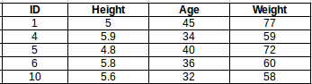
Let’s start with a simple example. Consider the table below—it includes the height, age, and weight (target) of 10 individuals. As shown, the weight value for ID11 is missing. Below, we need to predict this person’s weight based on their height and age.
Note: The data in this table does not represent actual values. It is just an example to explain this concept.

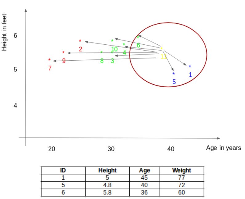
To clarify this further, here is the relationship graph between height and age derived from the above table:
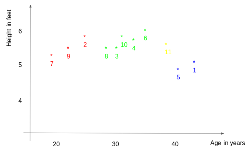
In the above graph, the y-axis represents a person’s height (in feet), and the x-axis represents age (in years). These points are numbered according to their ID values. The yellow point (ID 11) is our test point.
If you were to determine the weight of the person with ID11 based on the above graph, what would your answer be? You might say that because ID11 is closer to points 5 and 1, this person’s weight should be similar to these IDs, likely between 72-77 kg (the weights of IDs 1 and 5 in the table). This makes sense, but how does the algorithm predict these values? We will find the answer in this article.
2. How Does the KNN Algorithm Work?
As mentioned above, KNN can be used for both classification and regression problems. The algorithm uses “feature similarity” to predict the value of any new data point. This means assigning a value to the new point based on its similarity to points in the training set. From our example, we know that ID11’s height and age are similar to those of IDs 1 and 5, so their weights should also be roughly the same.
If this were a classification problem, we would take the mode as the final prediction. In this case, we have two weight values—72 and 77. Who can guess how the final value is calculated? We would take the average of the two values as the final prediction.
The specific steps of this algorithm are as follows:
First, calculate the distance between the new point and every point in the training set.
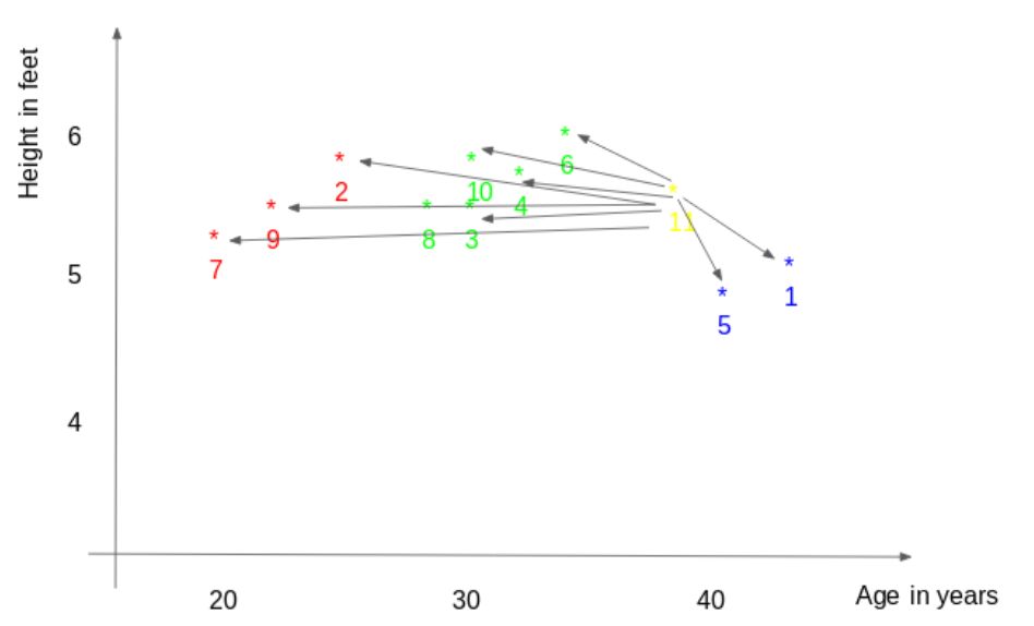
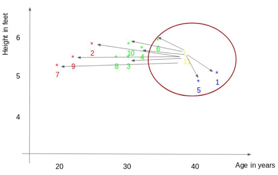
Select the K closest points to the new point (based on distance). In this example, if K=3, points 1, 5, and 6 would be selected. In the later sections of this article, we will further explore how to choose the correct K value.
Take the mean of all points as the final predicted value for the new point. In this example, we can get the weight of ID11 = (77+72+60)/3 = 69.66kg.
In the next few sections, we will discuss the specific details of the above three steps.
3. Methods for Calculating Distance Between Points
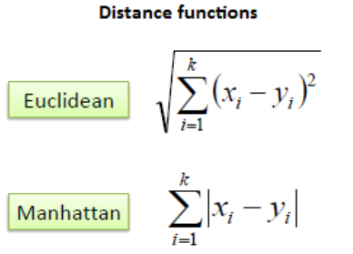
The first step is to calculate the distance between the new point and each point in the training set. There are many ways to calculate this distance, among which the most common methods are Euclidean distance, Manhattan distance (continuous), and Hamming distance (discrete).
-
Euclidean distance: The Euclidean distance is the square root of the sum of the squared differences between the new point (x) and the existing point (y).
-
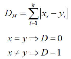
Manhattan distance: This is the distance between real vectors, calculated by the sum of their absolute differences.
-
Hamming distance: Used for discrete variables, if (x) and (y) values are equal, the distance D equals 0. Otherwise, D = 1.
Once the distance between the new observation point and the points in the training set is calculated, the next step is to select the nearest points. The number of points is determined by the K value.
4. How to Choose the K Factor?
The second step is to determine the K value. When assigning a value to the new observation point, the K value determines the number of neighboring points to be referenced.
In our example, for K=3, the closest points are ID1, ID5, and ID6.
The predicted weight for ID11 is:
ID11 = (77+72+60)/3
ID11 = 69.66 kg
For k=5, the closest points are ID1, ID4, ID5, ID6, and ID10.
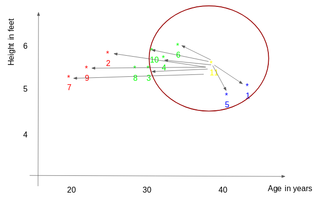
The predicted weight for ID11 is:
ID 11 = (77+59+72+60+58)/5
ID 11 = 65.2 kg
We notice that, depending on the K value, the final result often changes. So how do we find the optimal value of K? Let’s determine it based on the training and validation set errors. (After all, minimizing error is our ultimate goal!)
Please see the chart below for training and validation errors for different K values.
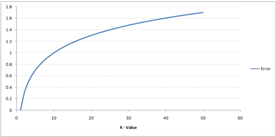
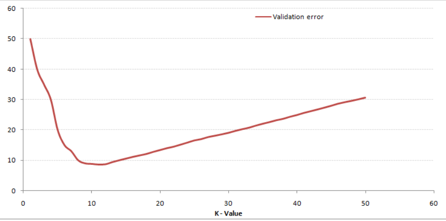
When K is low (assuming K = 1), the model overfits the training data, resulting in a high error rate on the validation set. On the other hand, when K takes a large value, the model performs poorly on both the training and validation sets. If you observe closely, the value of the validation error curve reaches its minimum at K = 9, at which point the K value is the optimal value for the model (this will vary depending on the dataset). This curve is called the “elbow curve” (because its shape resembles an elbow) and is often used to determine the K value.
We can also use grid search techniques to determine the K value. In the next section, we will introduce it.
5. Application on a Dataset
By now, you should have a clear understanding of the algorithm. If you have any questions, please leave a message on our public account; we are happy to answer. Now, we will implement the algorithm on a dataset. I have used the Big Mart sales dataset to demonstrate the implementation process; you can download it from this link.
-
Reading the file
import pandas as pd
df = pd.read_csv(‘train.csv’)
df.head()
-
Calculating missing values
df.isnull().sum()
#missing values in Item_weight and Outlet_size need to be imputed
mean = df[‘Item_Weight’].mean() #imputing item_weight with mean
df[‘Item_Weight’].fillna(mean, inplace =True)
mode = df[‘Outlet_Size’].mode() #imputing outlet size with mode
df[‘Outlet_Size’].fillna(mode[0], inplace =True)
-
Processing categorical variables, removing ID columns
df.drop([‘Item_Identifier’, ‘Outlet_Identifier’], axis=1, inplace=True)
df = pd.get_dummies(df)
-
Creating training and testing sets
from sklearn.model_selection import train_test_split
train , test = train_test_split(df, test_size = 0.3)
x_train = train.drop(‘Item_Outlet_Sales’, axis=1)
y_train = train[‘Item_Outlet_Sales’]
x_test = test.drop(‘Item_Outlet_Sales’, axis = 1)
y_test = test[‘Item_Outlet_Sales’]
-
Preprocessing—Feature Scaling
from sklearn.preprocessing import MinMaxScaler
scaler = MinMaxScaler(feature_range=(0, 1))
x_train_scaled = scaler.fit_transform(x_train)
x_train = pd.DataFrame(x_train_scaled)
x_test_scaled = scaler.fit_transform(x_test)
x_test = pd.DataFrame(x_test_scaled)
-
Checking the error rates for different K values
#import required packages
from sklearn import neighbors
from sklearn.metrics import mean_squared_error
from math import sqrt
import matplotlib.pyplot as plt
%matplotlib inline
rmse_val = [] #to store rmse values for different k
for K in range(20):
K = K+1
model = neighbors.KNeighborsRegressor(n_neighbors = K)
model.fit(x_train, y_train) #fit the model
pred=model.predict(x_test) #make prediction on test set
error = sqrt(mean_squared_error(y_test,pred)) #calculate rmse
rmse_val.append(error) #store rmse values
print(‘RMSE value for k= ‘ , K , ‘is:’, error)
Output:
RMSE value for k = 1 is: 1579.8352322344945
RMSE value for k = 2 is: 1362.7748806138618
RMSE value for k = 3 is: 1278.868577489459
RMSE value for k = 4 is: 1249.338516122638
RMSE value for k = 5 is: 1235.4514224035129
RMSE value for k = 6 is: 1233.2711649472913
RMSE value for k = 7 is: 1219.0633086651026
RMSE value for k = 8 is: 1222.244674933665
RMSE value for k = 9 is: 1219.5895059285074
RMSE value for k = 10 is: 1225.106137547365
RMSE value for k = 11 is: 1229.540283771085
RMSE value for k = 12 is: 1239.1504407152086
RMSE value for k = 13 is: 1242.3726040709887
RMSE value for k = 14 is: 1251.505810196545
RMSE value for k = 15 is: 1253.190119191363
RMSE value for k = 16 is: 1258.802262564038
RMSE value for k = 17 is: 1260.884931441893
RMSE value for k = 18 is: 1265.5133661294733
RMSE value for k = 19 is: 1269.619416217394
RMSE value for k = 20 is: 1272.10881411344
#plotting the rmse values against k values
curve = pd.DataFrame(rmse_val) #elbow curve
curve.plot()
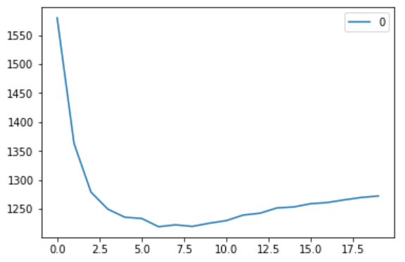
As we discussed, when k=1, we get a very high RMSE value. The RMSE value decreases as the K value increases. At k=7, the RMSE is approximately 1219.06, and it further increases with higher K values. We can confidently say that K=7 yields the best results in this case.
These are the predicted results obtained using the training dataset. Now let’s predict the values for the test dataset and submit.
-
Getting predicted values on the test set
#reading test and submission files
test = pd.read_csv(‘test.csv’)
submission = pd.read_csv(‘SampleSubmission.csv’)
submission[‘Item_Identifier’] = test[‘Item_Identifier’]
submission[‘Outlet_Identifier’] = test[‘Outlet_Identifier’]
#preprocessing test dataset
test.drop([‘Item_Identifier’, ‘Outlet_Identifier’], axis=1, inplace=True)
test[‘Item_Weight’].fillna(mean, inplace =True)
test = pd.get_dummies(test)
test_scaled = scaler.fit_transform(test)
test = pd.DataFrame(test_scaled)
#predicting on the test set and creating submission file
predict = model.predict(test)
submission[‘Item_Outlet_Sales’] = predict
submission.to_csv(‘submit_file.csv’,index=False)
By submitting this file, I obtained an RMSE of 1279.5159651297.
-
Implementing Grid Search
To determine the K value, plotting the elbow curve each time is a tedious process. We can simply use grid search to find the best value.
from sklearn.model_selection import GridSearchCV
params = {‘n_neighbors’:[2,3,4,5,6,7,8,9]}
knn = neighbors.KNeighborsRegressor(
model = GridSearchCV(knn, params, cv=5)
model.fit(x_train,y_train)
model.best_params
Output:
{‘n_neighbors’: 7}
6. Additional Resources
In this article, we introduced the working principle of the KNN algorithm and its implementation in Python. This is one of the most basic and effective machine learning techniques. For implementing KNN in R, you can browse this article: KNN Algorithm in R.
In this article, we directly used the KNN model from the sklearn library. You can also implement KNN from scratch (which I recommend doing!), and this article will cover that: KNN Simplified.
If you think you know KNN well and have a solid grasp of the technique, test your skills in this MCQ quiz: 30 Questions on KNN Algorithm. Good luck!
Translator’s Note: Process for Registering to Download the Dataset
1. Register an account, then sign up for this competition

2. Click ondata

Then you can happily download, run, and test~

The translator’s score is:

Feel free to leave your scores and insights~
Reply with“1119” to get relevant links.
Original Title:
A Practical Introduction to K-Nearest Neighbors Algorithm for Regression (with Python code)
Original Link:
https://www.analyticsvidhya.com/blog/2018/08/k-nearest-neighbor-introduction-regression-python/
Translator’s Profile

ZHAO XUEYAO, currently a graduate student at Beijing University of Posts and Telecommunications, an intern algorithm engineer at JD.com, currently researching reinforcement learning advertising bidding models. I believe that data and algorithms will empower enterprise development, and I hope to explore cutting-edge news and delve into the limits of algorithms with like-minded partners. On the path of hyperparameter tuning, I run all the way.
Recruitment Information for Translation Team
Job Description: Requires a meticulous heart to translate selected foreign articles into fluent Chinese. If you are a graduate student in data science/statistics/computer science, or working overseas in related fields, or confident in your language skills, you are welcome to join the translation team.
What You Will Get: Regular translation training to improve volunteers’ translation skills, enhance awareness of cutting-edge data science, and overseas friends can keep in touch with domestic technology application development. The THU Data Team’s background in industry-university-research provides good development opportunities for volunteers.
Other Benefits: You will have the chance to work with data scientists from well-known companies, as well as students from prestigious universities like Peking University, Tsinghua University, and overseas schools; they will become your partners in the translation team.
Click on the “Read Original” at the end of the article to join the Data Team~
Reprinting Instructions
If you need to reprint, please indicate the author and source prominently at the beginning (reprinted from: Data Team ID: datapi), and place the Data Team’s prominent QR code at the end of the article. For articles with original identification, please send [Article Name – Pending Authorization Public Account Name and ID] to the contact email to apply for whitelist authorization and edit according to requirements.
After publishing, please provide the link to the contact email (see below). Unauthorized reprints and adaptations will be pursued legally.


Click on “Read Original” to embrace the organization