
Author: Jeremy Jordan
Translation by Machine Heart
Contributors: Huang Xiaotian, Xu Di
Every machine learning researcher faces the challenge of hyperparameter tuning, and during this tuning process, the adjustment of the learning rate is a crucial part. The learning rate represents the speed at which information accumulates over time in a neural network. Ideally, we start with a large learning rate and gradually reduce it until the loss no longer diverges. However, this is easier said than done. The author of this article briefly introduces the thoughts on adjusting the learning rate, hoping it will be helpful to you.
In a previous article, I discussed how to train neural networks using backpropagation and gradient descent. One of the key hyperparameters that needs to be set for training a neural network is the learning rate. Just a reminder, this parameter scales the magnitude of weight updates to minimize the loss function of the network.
If you set the learning rate too low, training will progress very slowly because you make very few adjustments to the weights of the network. However, if your learning rate is set too high, it may lead to undesirable consequences on your loss function. I have visualized these cases—if you find these graphs difficult to understand, I recommend referring back to (at least) the first part of my previous post on gradient descent.
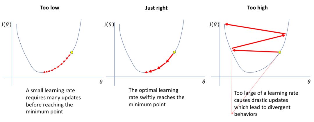
So, how do we find the optimal learning rate?
Let’s see what Tesla AI director and Andrej Karpathy’s protégé has to say:
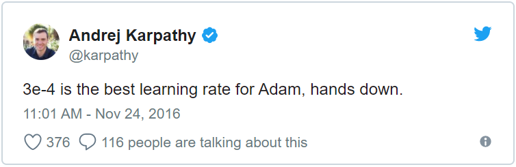
Tweet: 3e-4 is the best learning rate for Adam, for sure~
Perfect, I feel like my job is done
Well, not really…
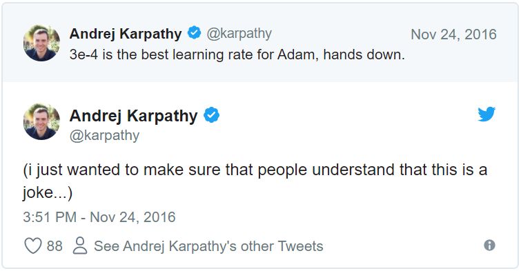
Second tweet: I want to confirm that everyone knows this is a joke, right…?
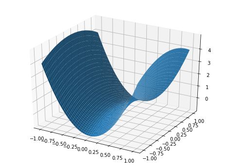
The loss function landscape of a neural network (as shown below) is a function of the values of the network parameters, quantifying the “error” associated with using a specific parameter configuration when performing inference (prediction) on a given dataset. This loss landscape can look very different for very similar network architectures. The image below is from the paper “Visualizing the Loss Landscape of Neural Nets,” which shows how residual connections can create smoother topologies.
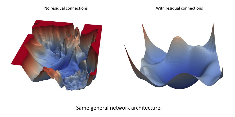
The optimal learning rate depends on the topology of your loss landscape, which is determined by your model structure and dataset. When you use a default learning rate (automatically determined by your deep learning library), it can provide a reasonably good result, and you can improve performance by searching for the optimal learning rate. I hope you find this easy in the next section.
A Systematic Approach to Finding the Optimal Learning Rate
Ultimately, we want to obtain a learning rate that significantly reduces network loss. We can observe and record the loss after each incremental increase in learning rate by gradually increasing the learning rate for each mini-batch (iteration) during a simple experiment. This gradual increase can be linear or exponential.
For too slow a learning rate, the loss function may decrease, but at a very shallow rate. When entering the optimal learning rate region, you will observe a significant drop in the loss function. Further increasing the learning rate will cause the loss function value to “bounce around” or even diverge near the minimum. Remember, the best learning rate corresponds to the steepest descent on the loss function, so we primarily focus on analyzing the slope of the graph.
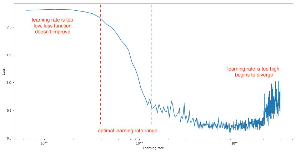
You should set your learning rate limits for this experiment so that you can see all three phases, ensuring the identification of the optimal range.
Setting a Schedule to Adjust Your Learning Rate During Training
Another commonly used trick is learning rate annealing, where it is recommended to start with a relatively high learning rate and then gradually reduce the learning rate during training. The idea behind this method is that we want to move quickly from the initial parameters to a parameter value that is “good,” but afterward, we want a learning rate small enough to explore “deeper and narrower places on the loss function” (from Karpathy’s CS231n course notes: http://cs231n.github.io/neural-networks-3/#annealing-the-learning-rate). If you find it hard to imagine what I just said, think back to how a high learning rate can cause parameter updates to “bounce around” between minima, leading to noisy convergence within a very small range, or in more extreme cases, diverging from the minimum altogether.
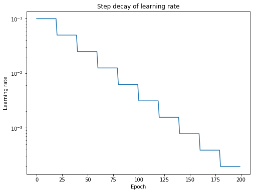
The most popular way to anneal the learning rate is through step decay, where the learning rate drops by a certain percentage after a specified number of training epochs.
More commonly, we can create a learning rate schedule, which updates the learning rate based on specific rules during training.
Cyclical Learning Rates
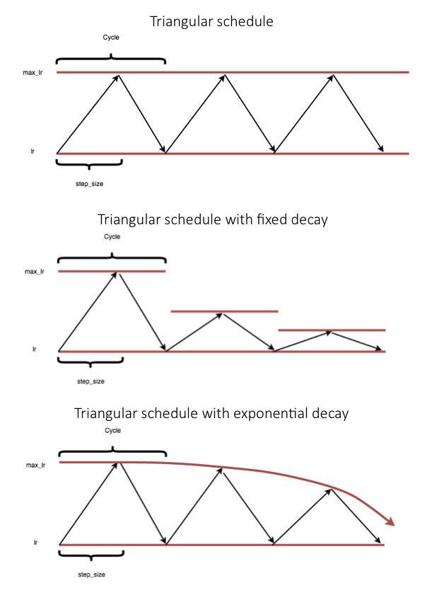
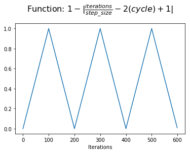
In the paper “Cyclical Learning Rates for Training Neural Networks,” Leslie Smith proposes a cyclical learning rate schedule that varies between two bounds. As shown in the figure below, it follows a triangular update rule, but he also mentions how to combine this rule with fixed period decay or exponential period decay.
Note: At the end of this article, I will provide the code to implement this learning rate. Therefore, if you are not interested in understanding the mathematical formulas, you can skip that part.
We can write it as:

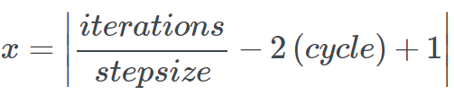
Where x is defined as
And cycle is calculated as
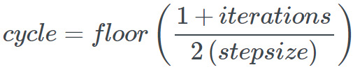
Where η_min and η_max define the bounds of the learning rate, iterations represent the number of mini-batches completed, and stepsize defines half the length of a cycle. As far as I know, 1−x is always positive, so the max operation does not seem absolutely necessary.
To understand how this equation works, let us build it step by step using visualization. For the visual effect below, triangular updates for three complete cycles are shown with a step length of 100 iterations. Remember, one iteration corresponds to one mini-batch of training.
Most importantly, we can determine the “progress” during training based on the number of half-cycles completed. We measure our progress in half-cycles rather than full cycles, allowing for symmetry within a cycle (you will understand this point more clearly later).
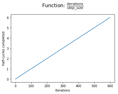
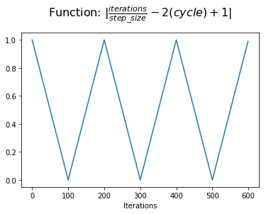
Next, we compare the half-cycle progress with the number of half-cycles completed at the end of the current cycle. At the start of a cycle, we have two half-cycles to complete; by the end of a cycle, this value reaches zero.
Next, we add 1 to this value, shifting the function to center around the y-axis. Now we refer to half-cycle points to display progress within a cycle.

At this point, we take the absolute value to complete a triangle within each cycle. This is the value we assign to x.
However, we want the learning rate schedule to start from a minimum, increase to a maximum in the middle of the cycle, and then drop back to the minimum. We can achieve this by simply calculating 1-x.
By adding a portion of the learning rate range to the minimum learning rate (also known as the base learning rate), we now have a value that can adjust the learning rate.
Smith writes that the main theoretical assumption behind cyclical learning rates (as opposed to reducing learning rates) is that “increasing the learning rate may have a short-term negative effect, but it leads to long-term positive effects.” Indeed, his paper includes several examples of loss function evolution, which temporarily deviate to higher losses compared to a fixed learning rate baseline and ultimately converge to lower losses.
To intuitively understand how this short-term impact leads to long-term positive effects, it is important to understand the expected characteristics of our convergence minima. Ultimately, we want our network to learn from the data in a way that generalizes to unseen data. Consequently, a network with good generalization capabilities should be robust, where small changes in parameters do not significantly impact performance. Given this, it is reasonable that sharp minima lead to poor generalization, as small changes in parameter values can lead to significantly higher losses. By allowing our learning rate to increase in iterations, we can “jump out” of sharp minima, which may temporarily increase loss but could ultimately converge to more desirable minima.
Note: Although “proper minima for good generalization” is widely accepted, there are also strong counterarguments (https://arxiv.org/abs/1703.04933).
Additionally, increasing the learning rate allows for “faster traversal across saddle point plateaus.” As seen in the figure below, gradients can be very small at saddle points. Because parameter updates are a gradient function, this leads to very short optimization steps; increasing the learning rate here can help avoid getting stuck at saddle points for too long, which is useful.

Note: By definition, a saddle point is a critical point where some dimensions observe local minima while others observe local maxima. Due to neural networks having thousands or millions of parameters, it is unrealistic to observe a true local minimum across all dimensions; this is the significance of saddle points. When I mention “sharp minima,” we should actually depict a saddle point where the minima dimensions are very steep and the maxima dimensions are very broad (as shown in the figure below).
Stochastic Gradient Descent with Warm Restarts (SGDR)
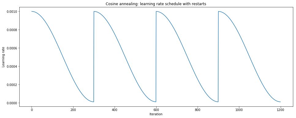
Stochastic Gradient Descent with Warm Restarts (SGDR) is similar to the cyclical method, where a positive annealing schedule is combined with periodic “restarts” back into the original initial learning rate.
We can write it as
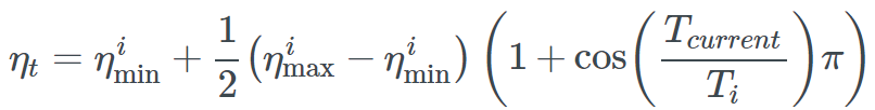
Where η_t is the learning rate at time step t (increased between each mini-batch) and
and defines the ideal range of learning rates, T_current represents the number of epochs since the last restart, and T_i defines the number of epochs within a cycle. Let’s try to break down this equation.
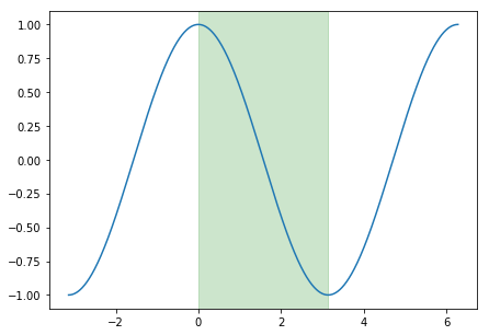
This annealing schedule relies on the cosine function, which varies between -1 and 1. It can take values between 0 and 1, which is the input to our cosine function. The corresponding area of the cosine function is highlighted in green in the figure below. By adding 1, our function varies between 0 and 2, then scaling down by 1/2, it varies between 0 and 1. Thus, we simply take the minimum learning rate and add a portion of the specified learning rate range. Since this function starts from 1 and decreases to 0, the result is a learning rate that starts from a maximum within a specified range and decays to a minimum. Once our cycle ends, T_current resets to 0, and we restart this process from the maximum learning rate.
The author also found that this learning rate schedule can be applied to:
-
Extending cycles as training progresses
-
Decay after each cycle
 and
and
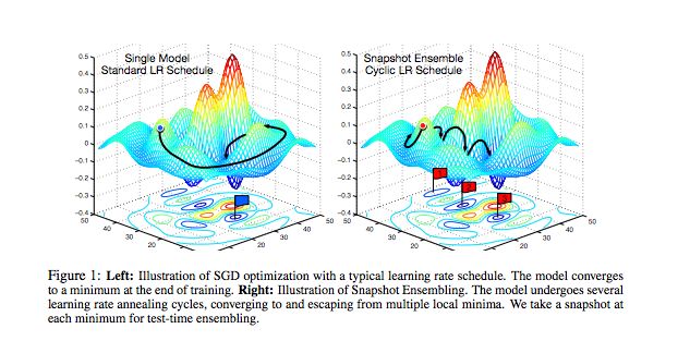
By thoroughly increasing the learning rate at each restart, we can essentially exit a local low point and continue exploring the loss landscape.
Very cool idea: After each round of cycles, snapshot the weights; researchers can build a full set of models by training a single model. This is because from one cycle to another, the network “settles” in different local optima, as illustrated in the figure below.
Implementation
Finding the optimal learning rate and setting a learning rate schedule can be easily applied using Keras callback functions.
Finding the Optimal Learning Rate Range
We can write a Keras callback function that tracks the loss function in conjunction with a linearly changing learning rate within a specified range.
from keras.callbacks import Callback
import matplotlib.pyplot as plt

class LRFinder(Callback):

    '''
    A simple callback for finding the optimal learning rate range for your model + dataset.

    # Usage

        ```python
            lr_finder = LRFinder(min_lr=1e-5, max_lr=1e-2, steps_per_epoch=10, epochs=3)
            model.fit(X_train, Y_train, callbacks=[lr_finder])

            lr_finder.plot_loss()
        ```

    # Arguments
        min_lr: The lower bound of the learning rate range for the experiment.
        max_lr: The upper bound of the learning rate range for the experiment.
        steps_per_epoch: Number of mini-batches in the dataset.
        epochs: Number of epochs to run experiment. Usually between 2 and 4 epochs is sufficient.

    # References

        Blog post: jeremyjordan.me/nn-learning-rate
        Original paper: https://arxiv.org/abs/1506.01186
    '''

    def __init__(self, min_lr=1e-5, max_lr=1e-2, steps_per_epoch=None, epochs=None):
        super().__init__()

        self.min_lr = min_lr
        self.max_lr = max_lr
        self.total_iterations = steps_per_epoch * epochs
        self.iteration = 0
        self.history = {}

    def clr(self):
        '''Calculate the learning rate.'''
        x = self.iteration / self.total_iterations
        return self.min_lr + (self.max_lr-self.min_lr) * x

    def on_train_begin(self, logs=None):
        '''Initialize the learning rate to the minimum value at the start of training.'''
        logs = logs or {}
        K.set_value(self.model.optimizer.lr, self.min_lr)

    def on_batch_end(self, epoch, logs=None):
        '''Record previous batch statistics and update the learning rate.'''
        logs = logs or {}
        self.iteration += 1

        K.set_value(self.model.optimizer.lr, self.clr())

        self.history.setdefault('lr', []).append(K.get_value(self.model.optimizer.lr))
        self.history.setdefault('iterations', []).append(self.iteration)

        for k, v in logs.items():
            self.history.setdefault(k, []).append(v)

    def plot_lr(self):
        '''Helper function to quickly inspect the learning rate schedule.'''
        plt.plot(self.history['iterations'], self.history['lr'])
        plt.yscale('log')
        plt.xlabel('Iteration')
        plt.ylabel('Learning rate')

    def plot_loss(self):
        '''Helper function to quickly observe the learning rate experiment results.'''
        plt.plot(self.history['lr'], self.history['loss'])
        plt.xscale('log')
        plt.xlabel('Learning rate')
        plt.ylabel('Loss')
Setting a Learning Rate Schedule
Step Decay
For a simple step decay, we can use the LearningRateScheduler callback.
import numpy as np
from keras.callbacks import LearningRateScheduler

def step_decay_schedule(initial_lr=1e-3, decay_factor=0.75, step_size=10):
    '''
    Wrapper function to create a LearningRateScheduler with step decay schedule.
    '''
    def schedule(epoch):
        return initial_lr * (decay_factor ** np.floor(epoch/step_size))

    return LearningRateScheduler(schedule)

lr_sched = step_decay_schedule(initial_lr=1e-4, decay_factor=0.75, step_size=2)

model.fit(X_train, Y_train, callbacks=[lr_sched])
Cyclical Learning Rates
To apply the cyclical learning rate technique, we can refer to this repo (https://github.com/bckenstler/CLR), which has implemented this technique from the paper. In fact, this repo has been cited in the paper’s appendix.
Stochastic Gradient Descent with Restarts
To apply this SGDR technique, we can refer to: https://github.com/keras-team/keras/pull/3525/files 
Original link: https://www.jeremyjordan.me/nn-learning-rate/
This article is translated by Machine Heart, please contact this public account for authorization to reprint.
✄————————————————
Join Machine Heart (Full-time Reporter/Intern): [email protected]
Submissions or inquiries: [email protected]
Advertising & Business Cooperation: [email protected]