 Source: New IntelligenceThis article is approximately 9000 words, and it is recommended to read for 10+minutes
This article takes you through the origins of artificial intelligence theory and the evolution of deep learning.
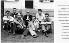
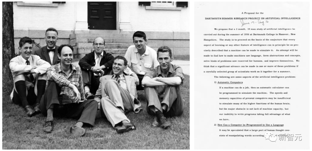
The term “artificial intelligence” was first officially proposed at the Dartmouth Conference in 1956 by John McCarthy and others.
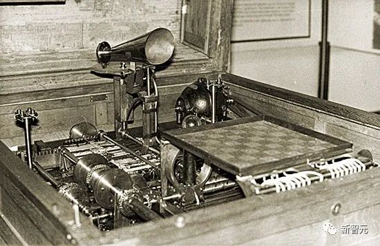
The concept of practical AI can be traced back to 1914 when Leonardo Torres y Quevedo constructed the first working chess machine that could play as a terminal game player. At that time, chess was considered an activity limited to intelligent beings.
As for the theory of artificial intelligence, it can be traced back to 1931-34 when Kurt Gödel established fundamental limits for any type of computation-based artificial intelligence.
As we move to the 1980s, the history of AI at this time emphasized topics such as theorem proving, logic programming, expert systems, and heuristic search.
The early 2000s AI history placed even more emphasis on themes such as support vector machines and kernel methods. Bayesian reasoning and other concepts from probability and statistics, decision trees, ensemble methods, swarm intelligence, and evolutionary computation drove many successful AI applications.
The 2020s AI research has become more “retro”, emphasizing concepts such as the chain rule and deep nonlinear artificial neural networks trained through gradient descent, particularly feedback-based recurrent networks.
Schmidhuber states that this article corrects the misleading “history of deep learning” that has been previously presented. In his view, most of the pioneering work mentioned in this article has been overlooked.
Moreover, Schmidhuber also refutes a common misconception that neural networks “as tools to help computers recognize patterns and simulate human intelligence were introduced in the 1980s”. In fact, neural networks appeared well before the 1980s.
1. 1676: The Chain Rule for Backpropagation
In 1676, Gottfried Wilhelm Leibniz published the chain rule of calculus in his memoirs. Today, this rule has become the core of credit assignment in deep neural networks, forming the foundation of modern deep learning.
Gottfried Wilhelm Leibniz
Neural networks have nodes or neurons that compute differentiable functions of inputs from other neurons, which in turn compute differentiable functions of inputs from other neurons. If one wants to know how changes in parameters or weights of earlier functions affect the final function output, the chain rule is needed.
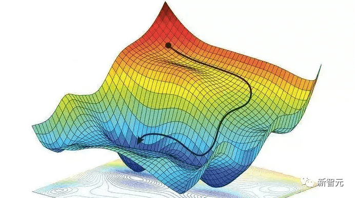
This answer is also used in gradient descent techniques. To teach neural networks to transform input patterns from the training set into desired output patterns, all neural network weights are iteratively adjusted towards maximum local improvement to create slightly better neural networks, and so forth, gradually approaching the optimal combination of weights and biases to minimize the loss function.
It is worth noting that Leibniz was also the first mathematician to discover calculus. He and Isaac Newton independently discovered calculus, and the mathematical symbols he used for calculus have become more widely used, with Leibniz’s symbols being generally considered more comprehensive and broadly applicable.
Additionally, Leibniz is also considered “the world’s first computer scientist”. In 1673, he designed the first machine capable of performing all four arithmetic operations, laying the foundation for modern computer science.
2. Early 19th Century: Neural Networks, Linear Regression, and Shallow Learning
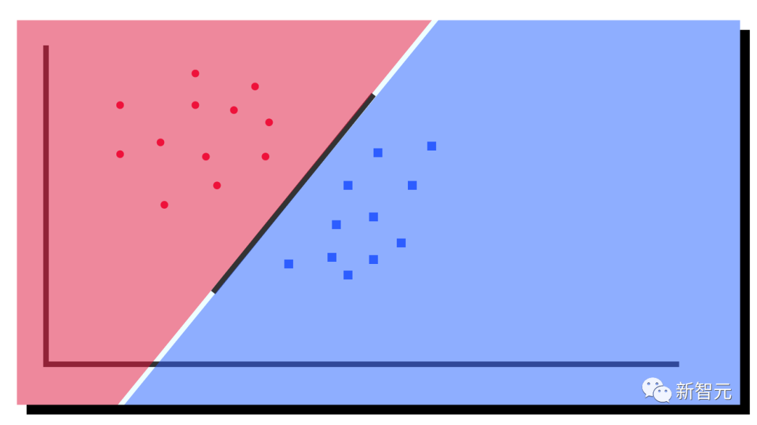
In 1805, Adrien-Marie Legendre published what is now commonly referred to as linear neural networks.
Adrien-Marie Legendre
Later, Johann Carl Friedrich Gauss was also recognized for similar research.
This neural network from over two centuries ago had two layers: an input layer with multiple input units and an output layer. Each input unit could hold a real number value and was connected to the output through connections with real-valued weights.
The output of the neural network is the sum of the products of the inputs and their weights. Given a training set of input vectors and the expected target value for each vector, the weights are adjusted to minimize the sum of the squared errors between the neural network output and the corresponding targets.
Of course, at that time it was not called a neural network. It was called the least squares method, also widely known as linear regression. But mathematically, it is the same as today’s linear neural networks: the same basic algorithm, the same error function, and the same adaptive parameters/weights.
Johann Carl Friedrich Gauss
This simple neural network performs “shallow learning”, in contrast to “deep learning” with many nonlinear layers. In fact, many neural network courses start by introducing this method before moving on to more complex and deeper neural networks.
Today, students from all technical disciplines must take mathematics courses, especially analysis, linear algebra, and statistics. In all these fields, many important results and methods can be attributed to Gauss: the fundamental theorem of algebra, Gaussian elimination, and the Gaussian distribution in statistics.
This “greatest mathematician of all time” also pioneered differential geometry, number theory (his favorite subject), and non-Euclidean geometry. Without his contributions, modern engineering, including AI, would be unimaginable.
3. 1920-1925: The First Recurrent Neural Network
Similar to the human brain, recurrent neural networks (RNNs) have feedback connections, allowing them to follow directed connections from some internal nodes to others, ultimately ending back at the starting point. This is crucial for remembering past events during sequence processing.
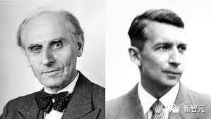
William Lenz (left); Ernst Ising (right)
Physicist Ernst Ising and William Lenz introduced and analyzed the first non-learning RNN architecture in the 1920s: the Ising model. It enters a balanced state based on input conditions, serving as the foundation for the first learning RNN model.
In 1972, Shun-Ichi Amari made the Ising model’s recurrent architecture adaptive, allowing it to learn by changing its connection weights to associate input patterns with output patterns. This was the world’s first learning RNN.
Shun-Ichi Amari
Currently, the most popular RNN is the Long Short-Term Memory network (LSTM) proposed by Schmidhuber. It has become the most cited neural network of the 20th century.
4. 1958: Multi-Layer Feedforward Neural Networks
In 1958, Frank Rosenblatt combined linear neural networks with threshold functions to design deeper multi-layer perceptrons (MLPs).
Frank Rosenblatt
Multi-layer perceptrons follow the principles of the human nervous system, learning and making predictions from data. They first learn, then store data using weights, and employ algorithms to adjust weights and reduce bias during training, i.e., the error between actual and predicted values.
Due to the frequent use of error backpropagation algorithms in training multi-layer feedforward networks, they are considered standard supervised learning algorithms in the field of pattern recognition and continue to be a subject of research in computational neuroscience and parallel distributed processing.
5. 1965: The First Deep Learning
The successful learning of deep feedforward network architectures began in 1965 in Ukraine when Alexey Ivakhnenko and Valentin Lapa introduced the first universal learning algorithm for deep MLPs with an arbitrary number of hidden layers.
Alexey Ivakhnenko
Given a training set of input vectors with corresponding target output vectors, the layers gradually increase in size and are trained through regression analysis, then pruned using a separate validation set where regularization is used to eliminate unnecessary units. The number of layers and units in each layer learn in a problem-relevant manner.
Like later deep neural networks, Ivakhnenko’s networks learned to create hierarchical, distributed, internal representations for incoming data.
He did not call them deep learning neural networks, but they were indeed so. In fact, the term “deep learning” was first introduced to machine learning by Dechter in 1986, while Aizenberg et al. introduced the concept of “neural networks” in 2000.
6. 1967-68: Stochastic Gradient Descent
In 1967, Shun-Ichi Amari first proposed training neural networks using Stochastic Gradient Descent (SGD).
Amari and his student Saito learned internal representations in a five-layer MLP with two modifiable layers, which were trained to classify non-linearly separable pattern classes.
Rumelhart, Hinton, and others did similar work in 1986 and named it the backpropagation algorithm.
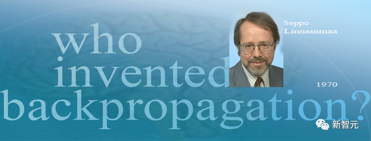
7. 1970: The Backpropagation Algorithm
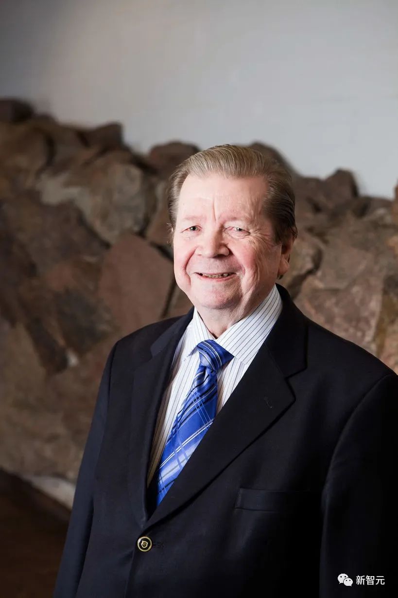
In 1970, Seppo Linnainmaa first published the backpropagation algorithm, a famous credit assignment algorithm for differentiable node networks, also known as “reverse mode of automatic differentiation”.
Seppo Linnainmaa
Linnainmaa first described an efficient way to propagate errors backward in class neural networks under arbitrary, discrete, sparse connections. It is now the foundation of widely used neural network software packages such as PyTorch and Google’s TensorFlow.
Backpropagation is essentially an effective way to implement Leibniz’s chain rule for deep networks. The gradient descent proposed by Cauchy gradually weakens certain neural network connections while strengthening others during many experimental processes.
By 1985, the computational cost had decreased by about 1,000 times compared to 1970, as desktop computers were just becoming popular in affluent academic laboratories. David Rumelhart and others conducted experimental analyses of known methods.
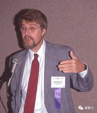
David Rumelhart
Through experiments, Rumelhart and others demonstrated that backpropagation could produce useful internal representations in the hidden layers of neural networks. At least for supervised learning, backpropagation is often more effective than the aforementioned deep learning performed by Amari using the SGD method.
Before 2010, many believed that training multi-layer neural networks required unsupervised pre-training. In 2010, Schmidhuber’s team, along with Dan Ciresan, demonstrated that deep FNNs could be trained through simple backpropagation without requiring unsupervised pre-training for significant applications.
8. 1979: The First Convolutional Neural Network
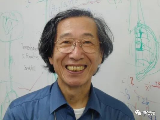
In 1979, Kunihiko Fukushima developed a neural network model for pattern recognition at STRL: the Neocognitron.

Kunihiko Fukushima
This Neocognitron, known today as a Convolutional Neural Network (CNN), is one of the greatest inventions of the basic structure of deep neural networks and is a core technology of current artificial intelligence.
The Neocognitron introduced by Dr. Fukushima was the first neural network to use convolution and downsampling, serving as a prototype for convolutional neural networks.
The artificial multi-layer neural network designed by Kunihiko Fukushima can mimic the visual network of the brain, and this “insight” has become the foundation of modern AI technology. Dr. Fukushima’s work has led to a series of practical applications, from autonomous vehicles to facial recognition, from cancer detection to flood prediction, with even more applications to come.
In 1987, Alex Waibel combined convolutional neural networks with weight sharing and backpropagation, proposing the concept of Time Delay Neural Networks (TDNN).
Since 1989, Yann LeCun’s team has contributed to the improvement of CNNs, especially in the field of images.

Yann LeCun
By the end of 2011, Schmidhuber’s team significantly accelerated the training speed of deep CNNs, making them more popular in the machine learning community. The team introduced a GPU-based CNN: DanNet, which was deeper and faster than earlier CNNs. That same year, DanNet became the first pure deep CNN to win a computer vision competition.
The Residual Neural Network (ResNet), proposed by four scholars from Microsoft Research, won the ImageNet Large Scale Visual Recognition Challenge in 2015.
Schmidhuber stated that ResNet is an early version of the fast neural networks (Highway Net) developed by his team. Compared to previous neural networks that had at most dozens of layers, this was the first truly effective deep feedforward neural network with hundreds of layers.
9. 1987-1990s: Graph Neural Networks and the Random Delta Rule
Deep learning architectures capable of manipulating structured data (e.g., graphs) were proposed by Pollack in 1987 and expanded and improved by Sperduti, Goller, and Küchler in the early 1990s. Today, graph neural networks are used in many applications.
Paul Werbos and R. J. Williams analyzed methods for implementing gradient descent in RNNs. Teuvo Kohonen’s Self-Organizing Maps also became popular.
Teuvo Kohonen
In 1990, Stephen Hanson introduced the Random Delta Rule, a stochastic method for training neural networks through backpropagation. Decades later, this method became popular under the nickname “dropout”.
10. February 1990: Generative Adversarial Networks / Curiosity
Generative Adversarial Networks (GANs) were first published in 1990 under the name “Artificial Intelligence Curiosity”.
Two adversarial neural networks (a probabilistic generator and a predictor) attempt to maximize each other’s loss in a minimax game. Among them:
- The generator (referred to as the controller) generates probabilistic outputs (using random units like later StyleGAN).
-
The predictor (referred to as the world model) observes the controller’s output and predicts how the environment will respond to them. Using gradient descent, the predictor NN minimizes its error while the generator NN attempts to maximize this error—one network’s loss is another network’s gain.
Four years before the 2014 paper on GANs, Schmidhuber summarized the generative adversarial NN from 1990 in the famous 2010 survey: “Neural networks predicting world models were used to maximize the controller’s intrinsic reward, which is proportional to the model’s prediction error.”
The GAN published later was merely an instance. The experiments were very brief, with the environment returning 1 or 0 based on whether the controller (or generator)’s output was in a given set.
The principles from 1990 have been widely used in reinforcement learning exploration and the synthesis of realistic images, although the latter field has recently been replaced by Latent Diffusion from Rombach et al.
In 1991, Schmidhuber published another ML method based on two adversarial NNs, called Predictability Minimization, used to create separable representations of partially redundant data, applied to images in 1996.
11. April 1990: Generating Subgoals / Working on Instructions
For centuries, most NNs have focused on simple pattern recognition rather than advanced reasoning.
However, in the early 1990s, exceptions began to emerge. This work injected the traditional “symbolic” hierarchical AI concept into end-to-end differentiable “sub-symbolic” NNs.
In 1990, Schmidhuber’s team’s NN learned to generate hierarchical action plans using an end-to-end differentiable NN subgoal generator for hierarchical reinforcement learning (HRL).
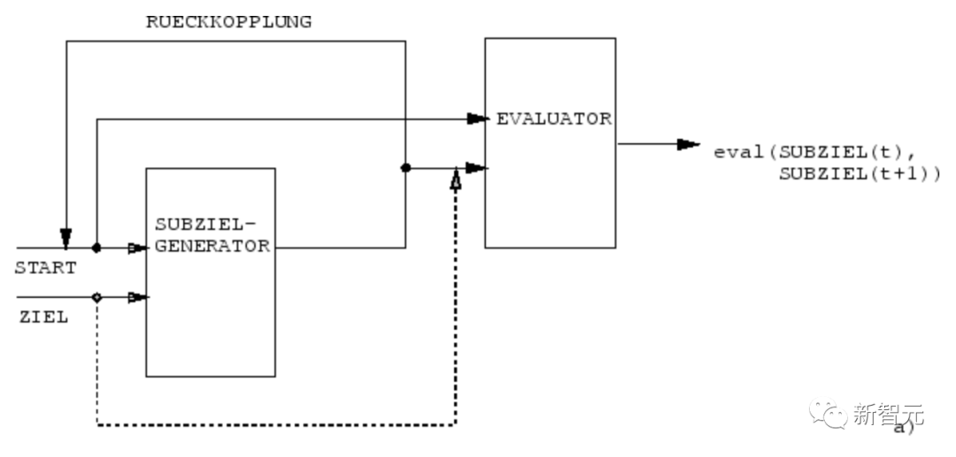
A reinforcement learning machine receives additional command inputs in the form of (start, goal). An evaluator NN learns to predict the current reward/cost from start to goal. A subgoal generator based on (R)NN also sees (start, goal) and learns a sequence of intermediate subgoals with minimal cost using the evaluator NN’s (copy) through gradient descent. The RL machine attempts to achieve the final goal using this sequence of subgoals.
The system learns action plans at multiple abstract levels and multiple time scales, in principle solving what has recently been called the “open-ended problem”.
12. March 1991: Transformer with Linear Self-Attention
The Transformer with “linear self-attention” was first published in March 1991.
These so-called “Fast Weight Programmers” or “Fast Weight Controllers” separated storage and control like traditional computers, but in an end-to-end differentiable, adaptive way, and as a neural network.
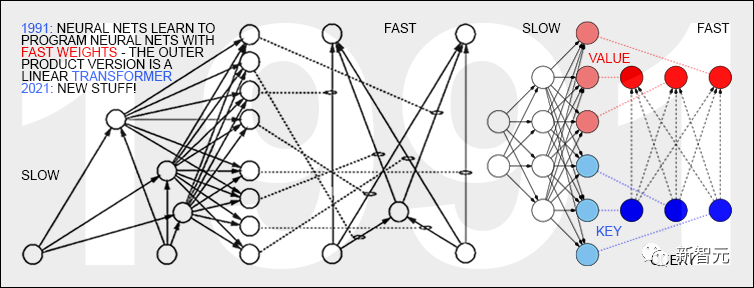
Moreover, today’s Transformers heavily utilize unsupervised pre-training, a deep learning method first published by Schmidhuber in 1990-1991.
13. April 1991: Distilling One NN into Another
Using the NN distillation procedure proposed by Schmidhuber in 1991, the hierarchical internal representation of the aforementioned neural history compressor can be compressed into a single recursive NN (RNN).
Here, the knowledge of the teacher NN is “distilled” into the student NN by training the student NN to mimic the teacher NN’s behavior (while also retraining the student NN to ensure that previously learned skills are not forgotten). The NN distillation method was also republished many years later and is widely used today.
14. June 1991: The Fundamental Problem – Vanishing Gradients
Sepp Hochreiter, Schmidhuber’s first student, discovered and analyzed the fundamental deep learning problem in his 1991 thesis.
Deep NNs suffer from the now-famous vanishing gradient problem: in typical deep or recurrent networks, the error signals from backpropagation either shrink rapidly or grow beyond limits. In both cases, learning fails.

15. June 1991: The Foundations of LSTM/Highway Net/ResNet
Long Short-Term Memory (LSTM) recurrent neural networks overcame the fundamental deep learning problems identified by Sepp Hochreiter in the aforementioned 1991 thesis.
After the peer-reviewed paper published in 1997 (now the most cited NN paper of the 20th century), Schmidhuber’s students Felix Gers, Alex Graves, and others further improved LSTM and its training procedures.
The LSTM variant with a forget gate, known as the “vanilla LSTM architecture”, published in 1999-2000, is still used today in Google’s TensorFlow.
In 2005, Schmidhuber first published papers on LSTM’s full backpropagation through time and bidirectional propagation (also widely used).

A milestone training method in 2006 was “Connectionist Temporal Classification” (CTC), used to align and recognize sequences simultaneously.
Schmidhuber’s team successfully applied CTC-trained LSTM to speech in 2007 (also with a layered LSTM stack), achieving outstanding end-to-end neural speech recognition results for the first time.
In 2009, thanks to Alex’s efforts, the CTC-trained LSTM became the first RNN to win an international competition, namely three ICDAR 2009 handwriting contests (French, Persian, Arabic). This sparked tremendous interest in the industry. LSTM was soon applied in all scenarios involving sequential data, such as speech and video.
In 2015, the combination of CTC-LSTM significantly improved Google’s speech recognition performance on Android smartphones. Until 2019, the speech recognition on Google mobile devices was still based on LSTM.
1995: Neural Probabilistic Language Models
In 1995, Schmidhuber proposed an excellent neural probabilistic text model, whose basic concept was reused in 2003.
In 2001, Schmidhuber showed that LSTM could learn languages that traditional models like HMM could not.
Google Translate in 2016 was based on two connected LSTMs (the white paper mentioned LSTM over 50 times), one for incoming text and one for outgoing translations.
That same year, over a quarter of the computing power used for inference in Google’s data centers was allocated to LSTM (with another 5% for another popular deep learning technique, namely CNN).
By 2017, LSTM also supported Facebook’s machine translation (over 30 billion translations per week), Apple’s Quicktype on about 1 billion iPhones, Amazon’s Alexa voice, Google’s image caption generation, and automatic email replies.
Of course, Schmidhuber’s LSTM has also been widely used in healthcare and medical diagnostics—simple Google Scholar searches can find countless titles with “LSTM” in medical articles.
In May 2015, Schmidhuber’s team proposed the Highway Network based on LSTM principles, the first very deep FNN with hundreds of layers (previous NNs had at most dozens of layers). Microsoft’s ResNet (which won the ImageNet 2015 competition) is one version of it.
The early Highway Net performed similarly to ResNet on ImageNet. Variants of Highway Net have also been used for certain algorithmic tasks where pure residual layers did not perform well.
The Principles of LSTM/Highway Net are Core to Modern Deep Learning
The core of deep learning is the depth of NNs.
In the 1990s, LSTM brought essentially unlimited depth to supervised RNNs; in 2000, inspired by LSTM, Highway Net brought depth to feedforward NNs.
Today, LSTM has become the most cited NN of the 20th century, while one version of Highway Net, ResNet, has become the most cited NN of the 21st century.
16. 1980 to Present: Learning Actions without Teachers in NNs
Furthermore, NNs are also related to reinforcement learning (RL).
While some problems can be solved using non-neural techniques invented as early as the 1980s, such as Monte Carlo tree search (MC), dynamic programming (DP), artificial evolution, α-β pruning, control theory, and system identification, deep FNNs and RNNs can yield better results for certain types of RL tasks.
Generally speaking, reinforcement learning agents must learn how to interact with a dynamic, initially unknown, partially observable environment without the help of teachers, maximizing the expected cumulative reward signal. There may be arbitrary, prior unknown delays between actions and perceivable outcomes.
When the environment has a Markov interface, making the inputs of the RL agent convey all the information needed to determine the next best action, RL based on dynamic programming (DP)/temporal difference (TD)/Monte Carlo tree search (MC) can be very successful.
For more complex situations without a Markov interface, agents must consider not only the current input but also the history of previous inputs. In this regard, the combination of RL algorithms and LSTM has become a standard solution, particularly through policy gradient training of LSTM.
For example, in 2018, an LSTM trained through PG was at the core of OpenAI’s famous Dactyl, which learned to control a dexterous robotic hand without teachers.
Video games are no different.
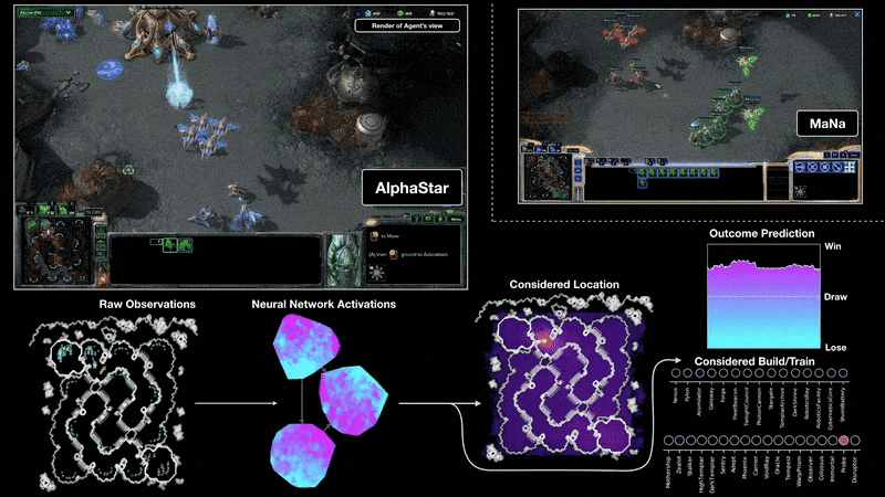
In 2019, DeepMind (co-founded by a student from Schmidhuber’s lab) defeated professional players in the game “StarCraft”, where the AI Alphastar utilized a deep LSTM core trained via PG.
Meanwhile, RL LSTM (which accounts for 84% of the total model parameters) is also at the core of the famous OpenAI Five, which defeated professional human players in Dota 2.
The future of RL will be about learning/combining/planning actions with compact spatiotemporal abstractions from complex input streams, which involves common sense reasoning and learning to think.
In the papers published by Schmidhuber in 1990-91, the self-supervised neural history compressor was proposed to learn hierarchical abstractions and representational concepts across multiple time scales; while the subgoal generator based on end-to-end differentiable NNs could learn hierarchical action plans through gradient descent.
In subsequent years, more complex methods for learning abstract thinking have been published in 1997 and 2015-18.
17. It’s a Hardware Problem, Fool!
Over the last thousand years, without the continuously improving and accelerating upgrades of computer hardware, deep learning algorithms could not have achieved significant breakthroughs.
The first known gear computing device is the Antikythera mechanism from ancient Greece over 2000 years ago. It is the oldest known complex scientific computer and the world’s first analog computer.

Antikythera Mechanism
The first practical programmable machine was invented by the ancient Greek mechanic Hero in the 1st century AD.
Machines became more flexible in the 17th century, capable of calculating answers based on input data.
The first mechanical calculator for simple arithmetic was invented by Wilhelm Schickard in 1623.
In 1673, Leibniz designed the first machine that could perform all four arithmetic operations and had memory. He also described the principle of a binary computer controlled by punched cards, which constitutes an important component of deep learning and modern artificial intelligence.

Leibniz Multiplier
Around 1800, Joseph Marie Jacquard and others in France manufactured the first programmable loom—the Jacquard machine. This invention played a crucial role in the future development of other programmable machines (such as computers).
Jacquard Loom
They inspired Ada Lovelace and her mentor Charles Babbage to invent a precursor to the modern electronic computer: Babbage’s Difference Engine.
In 1843, Lovelace published the world’s first computer algorithm.

Babbage’s Difference Engine
In 1914, the Spaniard Leonardo Torres y Quevedo became the first artificial intelligence pioneer of the 20th century, creating the first chess-playing terminal machine.
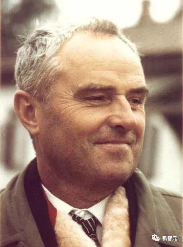
From 1935 to 1941, Konrad Zuse invented the world’s first operational programmable universal computer: the Z3.

Konrad Zuse
Unlike Babbage’s Analytical Engine, Zuse utilized Leibniz’s binary computing principles instead of traditional decimal computing, significantly simplifying the hardware load.
In 1944, Howard Aiken led a team to invent the world’s first large-scale automatic digital computer, the Mark I.
In 1948, Frederic Williams, Tom Kilburn, and Geoff Tootill invented the world’s first electronic stored-program computer: the Small Scale Experimental Machine (SSEM), also known as the “Manchester Baby”.

Replica of the “Manchester Baby”
Since then, computing has accelerated with the help of integrated circuits (ICs). In 1949, Siemens’ Werner Jacobi applied for a semiconductor patent for integrated circuits, allowing a single substrate to have multiple transistors.
In 1958, Jack Kilby demonstrated integrated circuits with external wires. In 1959, Robert Noyce proposed monolithic integrated circuits. Since the 1970s, graphics processing units (GPUs) have been used to accelerate computing through parallel processing. Today, computer GPUs contain billions of transistors.
Where Are the Physical Limits?
According to the Bremermann limit proposed by Hans Joachim Bremermann, a computer weighing 1 kilogram and occupying 1 liter can execute up to 10^51 operations per second at most 10^32 positions.
 Hans Joachim Bremermann
However, the mass of the solar system is only 2×10^30 kilograms, and this trend will inevitably break in a few centuries, as the speed of light will severely limit the acquisition of additional mass in other solar systems.
Thus, the constraints of physics require that future efficient computing hardware must have many compactly placed processors in three-dimensional space to minimize total connection costs, with its basic architecture essentially being a deep, sparsely connected three-dimensional RNN.
Schmidhuber speculates that deep learning methods for such RNNs will become increasingly important.
18. The Theory of Artificial Intelligence Since 1931
The core of modern AI and deep learning is primarily based on mathematics developed over the past few centuries: calculus, linear algebra, and statistics.
In the early 1930s, Gödel established modern theoretical computer science. He introduced a universal coding language based on integers, allowing the formalization of any digital computer’s operations in axiomatic form.
At the same time, Gödel constructed famous formal statements, systematically enumerating all possible theorems from a countable set of axioms through a given computational theorem verifier. Thus, he established fundamental limits for algorithmic theorem proving, computation, and any type of computation-based artificial intelligence.
Additionally, in his famous letter to John von Neumann, Gödel identified one of the most famous open problems in computer science: “P=NP?”.

In 1935, Alonzo Church derived a corollary of Gödel’s result by proving that Hilbert and Ackermann’s decision problem has no general solution. He used his other universal coding language, called Untyped Lambda Calculus, which forms the basis of the influential programming language LISP.
In 1936, Alan Turing introduced another universal model: the Turing machine, re-deriving the above results. That same year, Emil Post published another independent model of computation.
Konrad Zuse not only created the world’s first operational programmable universal computer but also designed the first high-level programming language—Plankalkül. He applied it to chess in 1945 and to theorem proving in 1948.

Plankalkül
Most of the early AI from the 1940s to 1970s was actually about theorem proving and Gödel-style deductions through expert systems and logic programming.
In 1964, Ray Solomonoff combined Bayesian (actually Laplace) probability reasoning with theoretical computer science to derive a mathematically optimal (but computationally infeasible) learning method for predicting future data from past observations.
He and Andrej Kolmogorov founded the theory of Kolmogorov complexity or algorithmic information theory (AIT), formalizing the concept of Occam’s razor by calculating the shortest program for the data, thus surpassing traditional information theory.

Kolmogorov Complexity
The self-reference Gödel machine’s more general optimality is not limited to asymptotic optimality.
Despite this, for various reasons, this mathematically optimal AI remains impractical. In contrast, practical modern AI is based on sub-optimal, limited, but not widely understood technologies, such as NNs and deep learning, which are the focus.
But who knows what the history of AI will look like in 20 years?
References:
https://people.idsia.ch/~juergen/deep-learning-history.html
Editor: Huang Jiyan