Author: Criss Source: Machine Learning and Generative Adversarial Networks
1.1 Derivative of Softmax
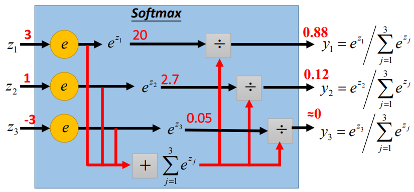
Generally, the last layer of a classification model is the softmax layer. Assuming we have a classification problem, the structure of the corresponding softmax layer is shown in the figure below (it is generally considered that the output result is the probability that the input belongs to class i):
Assuming a training set is given, the goal of the classification model is to maximize the log-likelihood function, which is
Generally, the optimization methods we adopt are gradient-based (e.g., SGD), meaning we need to solve . We only need to find , and then according to the chain rule, we can obtain , so our core task is to solve . From the above formula, we can see that we only need to know the of each sample to obtain by summation, and then through the chain rule, we can find . Therefore, we will omit the sample index j below and only discuss a certain sample .
In fact, there are two intuitive ways to represent which class belongs to:
-
One is the direct method (i.e., use to represent x belonging to class 3), then , where is the indicator function;
-
The other is the one-hot method (i.e., use to represent x belonging to class 3), then , where is the k-th element of the vector .
-
P.S., the one-hot method can also be understood as the implementation form of the direct method, because the one-hot vector is essentially .
For convenience, this article adopts the one-hot method. Thus, we have:
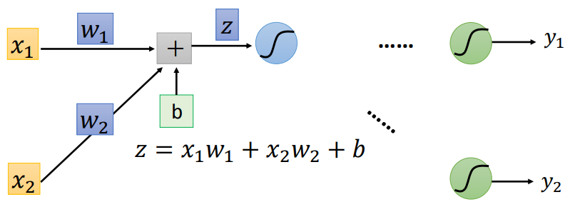
Additionally, let’s supplement the relationship between softmax and sigmoid. When the classification problem is binary, we generally use the sigmoid function as the output layer, representing the probability that the input belongs to class 1, that is
Then we use the probability sum of 1 to solve the probability that belongs to class 2, that is
At first glance, one might think that using sigmoid for binary classification is different from using softmax for binary classification:
-
When using softmax, the dimension of the output is consistent with the number of classes, while with sigmoid, the dimension of the output is less than the number of classes;
-
When using softmax, the probability expressions of the classes differ from those in sigmoid.
However, in fact, using sigmoid for binary classification is equivalent to using softmax for binary classification. We can make the output dimension of sigmoid consistent with the number of classes and approach softmax in form.
Through the above changes, sigmoid and softmax are already quite similar, except that the second element of the input for sigmoid is always equal to 0 (i.e., the input is ), while the input for softmax is . Below we will explain that there exists a mapping relationship between the two (i.e., each can find a corresponding to represent the same softmax result. However, it is worth noting that the reverse does not hold, meaning that not every corresponds to a single ).
Therefore, using sigmoid for binary classification is equivalent to using softmax for binary classification.
Generally, when training a neural network (i.e., updating the network parameters), we need the gradient of the loss function with respect to each parameter, and backpropagation is a method for calculating gradients.
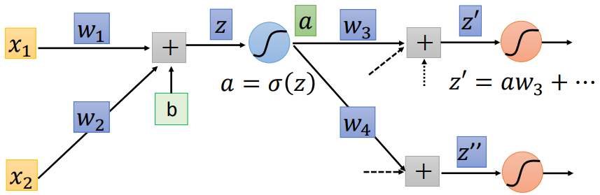
Assuming we have a neural network as shown in the figure above, and we want to find the gradient of the loss function with respect to , then according to the chain rule, we have
We can easily obtain the second term on the right side of the above equation, because , so we have
where is the output from the upper layer.
For the first term on the right side of the equation, we can further break it down as follows
We can easily obtain the second term on the right side of the above equation, because , and the activation function (e.g., sigmoid function) is defined by us, so we have
where is the linear output of this layer (before activation function).
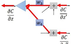
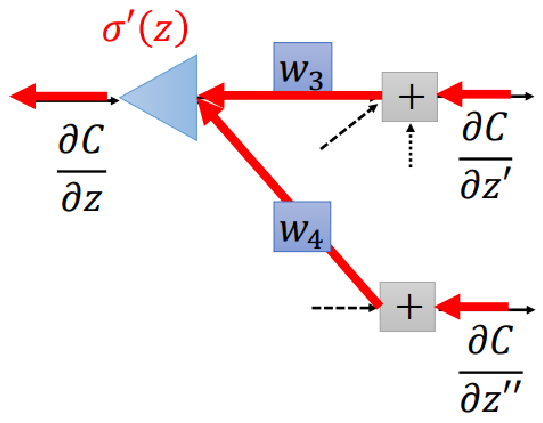
Observing the above figure, we can derive according to the chain rule
From we know that the values of and are known, so we are only left with and . Next, we adopt a dynamic programming (or recursive) approach. Assuming the values of the next layer’s and are known, we only need the gradient of the last layer to find the gradients of each layer. From the example of softmax, we know that the gradient of the last layer can indeed be calculated, so we can start from the last layer and move forward layer by layer to find the gradients of each layer.
Thus, the process of finding is actually corresponding to the neural network shown in the figure below (the reverse neural network of the original neural network):
In summary, we first perform forward computation through the neural network to obtain and , then find and ; then through backward computation of the neural network, we obtain and , and then find ; finally, we find according to the chain rule. This entire process is called backpropagation, where the forward computation process is called forward pass, and the backward computation process is called backward pass.
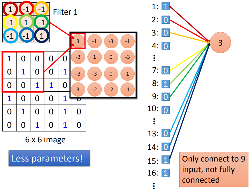
The convolutional layer is actually a special case of a fully connected layer, except that:
Some in the neurons are ;
Specifically, as shown in the figure below, no connection indicates that the corresponding w is 0:
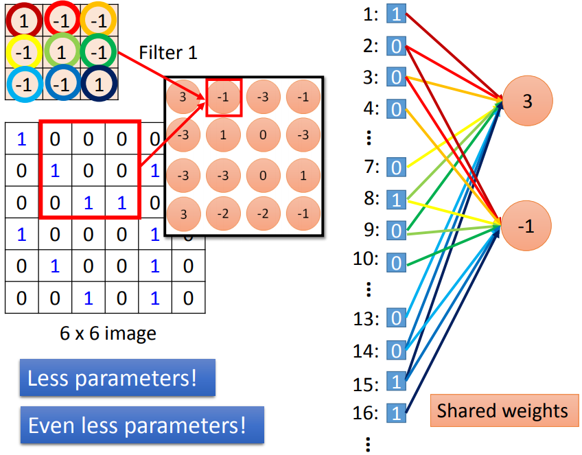
As shown in the figure below, the same color represents the same :
Therefore, we can understand the loss function as , and when deriving, according to the chain rule, we just need to add up the gradients of the same w, that is
When calculating each , we can treat them as independent , so it becomes the same as a regular fully connected layer, thus allowing us to use backpropagation for calculation.
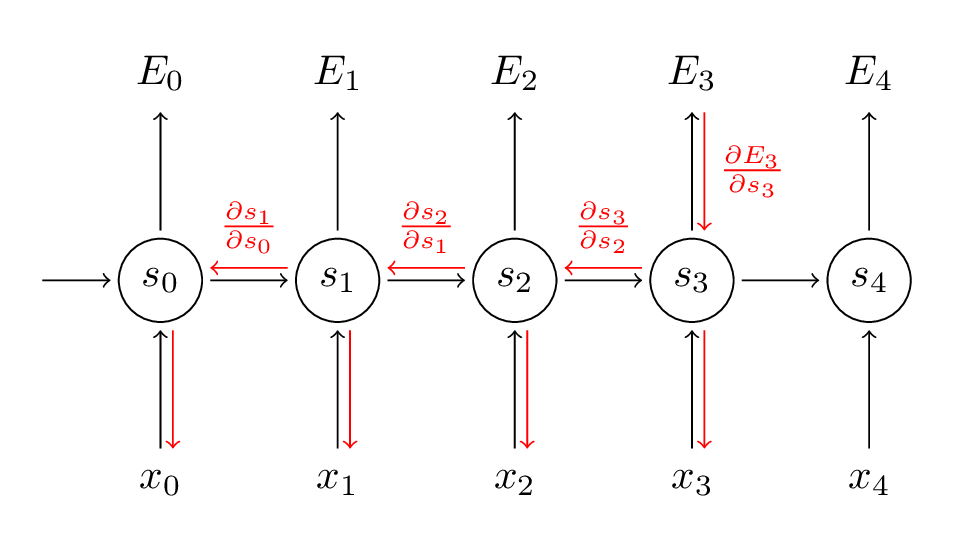
RNN unfolds over time as shown in the figure below (the red line indicates the gradient calculation route):
Like the approach used for convolutional layers, we first understand the loss function as , then treat each w as independent, and finally use the chain rule to find the corresponding gradient, that is
Since here, the RNN is unfolded into a neural network over time, this gradient calculation method is called Backpropagation Through Time (BPTT).
05 Derivative of Max Pooling
Generally, the function is non-differentiable, but if we already know which variable will be the maximum, then that function is differentiable (e.g., if we know y is the maximum, then the partial derivative with respect to y is 1, and for other variables, it is 0).
When training a neural network, we first perform a forward pass and then a backward pass, so when we derive max pooling, we already know which variable is the maximum, thus we can provide the corresponding gradient.
http://speech.ee.ntu.edu.tw/~tlkagk/courses_ML17_2.html
http://www.wildml.com/2015/10/recurrent-neural-networks-tutorial-part-3-backpropagation-through-time-and-vanishing-gradients/
Copyright Statement:Content sourced online, copyright belongs to the original authors.Unless unable to confirm, authors and sources will be indicated. If there is any infringement, please inform us, and we will delete and apologize immediately.Thank you!