5
A dataset typically refers to a two-dimensional array composed of several sample data, where each row represents the data of one sample.
For example: using gender, age, height (m), weight (kg), occupation, annual salary (ten thousand), real estate (ten thousand), and securities (ten thousand) to form a one-dimensional array representing the data of a marriage seeker, the following two-dimensional array is a dataset collected by a marriage agency.
import numpy as np
members = np.array([
  ['male', '25', 185, 80, 'programmer', 35, 200, 30],
  ['female', '23', 170, 55, 'civil servant', 15, 0, 80],
  ['male', '30', 180, 82, 'lawyer', 60, 260, 300],
  ['female', '27', 168, 52, 'journalist', 20, 180, 150]])
6
The columns of a dataset are also referred to as feature dimensions or feature columns.
The marriage seeker dataset above has a total of 8 columns: gender, age, height (m), weight (kg), occupation, annual salary (ten thousand), real estate (ten thousand), and securities (ten thousand), which can also be said to have 8 feature dimensions or feature columns.
Dimensionality reduction does not mean changing the dataset from two-dimensional to one-dimensional, but rather reducing the feature dimensions of the dataset.
The personal information of marriage seekers is far more than the 8 items listed above; it can also include birthday, hobbies, favorite colors, favorite foods, etc. However, if all personal information is added to the dataset, it will not only increase the difficulty and cost of data storage and processing, but also distract potential partners due to the excessive amount of information, leading them to overlook the most important information. Dimensionality reduction is about removing feature columns that have little or no impact on the results from the dataset.
Standardization is the process of centering each feature column of the sample set by subtracting the mean of that feature column and then scaling by dividing by the standard deviation.
In an exam with a full score of 100, if you scored 90, that is naturally a good grade. However, if compared to other students, it may not be: if all other students scored full marks, then 90 would be the worst. The significance of data standardization is to reflect the degree to which individual data deviates from the average of all samples. Below is the result of standardizing the securities feature column in the marriage seeker dataset.
security = np.float32((members[:,-1])) # Extract securities feature column data
(security - security.mean())/security.std() # Subtract mean and divide by standard deviation
9
Normalization is the process of centering each feature column of the sample set by subtracting the minimum value of that feature column and then scaling by dividing by the range (the difference between the maximum and minimum values).
Normalization is similar to standardization, with the results converging within the range of [0,1]. Below is the result of normalizing the securities feature column in the marriage seeker dataset.
security = np.float32((members[:,-1])) # Extract securities feature column data
(security - security.min())/(security.max() - security.min()) # Subtract min and divide by range
Machine learning models can only handle numerical data, so non-numerical data such as gender and occupation need to be converted to integers, a process known as feature encoding.
In the marriage seeker dataset, for the gender feature column, you can use 0 to represent female and 1 to represent male, or vice versa. However, this method is not suitable for encoding the occupation feature column, because different occupations are originally unordered; using this method would create a problem where 2 is closer to 1 than to 3. The common approach is to use one-hot encoding: if there are n different occupations, use n binary digits to represent them, where only one digit is 1 and the rest are 0. At this point, the occupation feature column will expand from 1 to n. Below, we use Scikit-learn’s one-hot encoder to encode the gender and occupation columns, generating 6 feature columns (2 for gender and 4 for occupation). This encoder is located in the preprocessing submodule.
from sklearn import preprocessing as pp
X = [
  ['male', 'programmer'],
  ['female', 'civil servant'],
  ['male', 'lawyer'],
  ['female', 'journalist'],
]
ohe = pp.OneHotEncoder().fit(X)
ohe.transform(X).toarray()
11
The datasets submodule in Scikit-learn provides several datasets: functions starting with load are built-in small datasets; functions starting with fetch need to download large datasets from external data sources.
datasets.load_boston([return_X_y]): Load the Boston housing price dataset
datasets.load_breast_cancer([return_X_y]): Load the Wisconsin breast cancer dataset
datasets.load_diabetes([return_X_y]): Load the diabetes dataset
datasets.load_digits([n_class, return_X_y]): Load the digits dataset
datasets.load_iris([return_X_y]): Load the iris dataset.
datasets.load_linnerud([return_X_y]): Load the physical training dataset
datasets.load_wine([return_X_y]): Load the wine dataset
datasets.fetch_20newsgroups([data_home, ...]): Load the news text classification dataset
datasets.fetch_20newsgroups_vectorized([...]): Load the vectorized news text dataset
datasets.fetch_california_housing([...]): Load the California housing dataset
datasets.fetch_covtype([data_home, ...]): Load the forest cover dataset
datasets.fetch_kddcup99([subset, data_home, ...]): Load the network intrusion detection dataset
datasets.fetch_lfw_pairs([subset, ...]): Load the face (paired) dataset
datasets.fetch_lfw_people([data_home, ...]): Load the face (labeled) dataset
datasets.fetch_olivetti_faces([data_home, ...]): Load the Olivetti face dataset
datasets.fetch_rcv1([data_home, subset, ...]): Load the Reuters English news text classification dataset
datasets.fetch_species_distributions([...]): Load the species distribution dataset
Each two-dimensional dataset corresponds to a one-dimensional label set, which is used to identify the category or attribute value of each sample. Typically, datasets are represented by uppercase letter X, and label sets by lowercase letter y.
The following code extracts the iris dataset from the datasets submodule – this is the most commonly used dataset for demonstrating classification models. The iris dataset X contains 150 samples, each with 4 feature columns: the length and width of the sepals and the length and width of the petals. There are 3 types of samples, represented by integers 0, 1, and 2, and all sample type labels form the label set y, which is a one-dimensional array.
from sklearn.datasets import load_iris
X, y = load_iris(return_X_y=True)
X.shape # The dataset X has 150 samples and 4 feature columns (150, 4)
y.shape # Each label in the label set y corresponds to each sample in dataset X (150,)
X[0], y[0](array([5.1, 3.5, 1.4, 0.2]), 0)
When loading data, if the return_X_y parameter is set to False (the default), you can view the names of the labels.
iris = load_iris()
iris.target_names # View the names of the labels
When training a model, the dataset and label set are usually divided into two parts: one part for training and one part for testing.
Splitting the dataset is a very important task, and different splitting methods have different impacts on the results of model training. Scikit-learn provides many dataset splitting methods, with train_test_split being one of the simplest, which can randomly extract a test set based on a specified ratio. The train_test_split function is located in the model_selection submodule.
from sklearn.datasets import load_iris
from sklearn.model_selection import train_test_split as tsplit
X, y = load_iris(return_X_y=True)
X_train, X_test, y_train, y_test = tsplit(X, y, test_size=0.1)
X_train.shape, X_test.shape((135, 4), (15, 4))
y_train.shape, y_test.shape((135,), (15,))
The above code randomly extracts samples as a test set from the dataset at a ratio of 10%, with the remaining samples as the training set. After the split, the training set has 135 samples, and the test set has 15 samples.
Like attracts like, and the nearest neighbor determines the category – this is k-nearest neighbors classification.
k-nearest neighbors classification is the simplest and easiest classification method. For a sample to be classified, find the k samples from the training set that are closest to it, and observe which label is most frequent among those samples, then assign that label to the sample to be classified. The best choice of k value highly depends on the data; a larger k value will suppress the influence of noise but will also make the classification boundaries less distinct. Typically, k values should be integers not greater than 20.
from sklearn.datasets import load_iris
from sklearn.model_selection import train_test_split as tsplit
from sklearn.neighbors import KNeighborsClassifier # Import k-nearest neighbors classification model
X, y = load_iris(return_X_y=True) # Get the iris dataset, returning samples and labels
X_train, X_test, y_train, y_test = tsplit(X, y, test_size=0.1) # Split into training set and test set
m = KNeighborsClassifier(n_neighbors=10) # Model instantiation, n_neighbors parameter specifies k value, default k=5
m.fit(X_train, y_train) # Model training
m.predict(X_test) # Classify the test set
array([2, 1, 2, 2, 1, 2, 1, 2, 2, 1, 0, 1, 0, 0, 2])
y_test # This is the actual classification situation, with only one error in the prediction
array([2, 1, 2, 2, 2, 2, 1, 2, 2, 1, 0, 1, 0, 0, 2])
m.score(X_test, y_test) # Model testing accuracy (between 0~1) 0.9333333333333333
Applying the classification model to classify 15 test samples, the result shows that only 1 is incorrect, with an accuracy of about 93%. In classification algorithms, score is the most commonly used evaluation function, returning the ratio of correctly classified samples to the total number of test samples.
How much can an 8-year-old Jeep Grand Cherokee be sold for? The simplest method is to refer to the average price of k used cars of the same model and similar usage years – this is k-nearest neighbors regression.
The k-nearest neighbors algorithm can be used to solve both classification and regression problems. In k-nearest neighbors regression, the predicted label of the sample is calculated as the average of the labels of its nearest neighbors. The following code demonstrates the usage of the k-nearest neighbors regression model using the Boston housing price dataset. The Boston housing price dataset records the median housing prices in the suburbs of Boston in the mid-1970s, with a total of 506 different data points, each containing 13 attributes such as the cultural, natural, and commercial environment, as well as traffic conditions, with the label being the average price of the area.
from sklearn.datasets import load_boston
from sklearn.model_selection import train_test_split as tsplit
from sklearn.neighbors import KNeighborsRegressor
X, y = load_boston(return_X_y=True) # Load the Boston housing price dataset
X.shape, y.shape, y.dtype # The dataset has 506 samples, 13 feature columns, and the label set is floating point, suitable for regression model((506, 13), (506,), dtype('float64'))
X_train, X_test, y_train, y_test = tsplit(X, y, test_size=0.01) # Split into training set and test set
m = KNeighborsRegressor(n_neighbors=10) # Model instantiation, n_neighbors parameter specifies k value, default k=5
m.fit(X_train, y_train) # Model training
m.predict(X_test) # Predict the prices of 6 test samples
array([27.15, 31.97, 12.68, 28.52, 20.59, 21.47])
y_test # This is the actual prices of the test samples, with the second sample (index 1) having a larger deviation, while the others are relatively acceptable
array([29.1, 50. , 12.7, 22.8, 20.4, 21.5])
Common evaluation methods for regression models include mean squared error, median absolute error, and coefficient of determination, among others.
Evaluating the quality of regression results is much more difficult than evaluating classification results – the former needs to consider the degree of deviation, while the latter only considers correctness. Common regression evaluation functions include mean squared error, median absolute error, and coefficient of determination, all of which are included in the metrics submodule for model evaluation. The smaller the mean squared error and median absolute error, the higher the precision of the model; conversely, the closer the coefficient of determination to 1, the higher the precision of the model, and the closer to 0, the less usable the model.
Taking the previous code as an example, the model evaluation results are as follows.
from sklearn import metrics

y_pred = m.predict(X_test)
metrics.mean_squared_error(y_test, y_pred) # Mean squared error 60.27319999999995
metrics.median_absolute_error(y_test, y_pred) # Median absolute error 1.0700000000000003
metrics.r2_score(y_test, y_pred) # Coefficient of determination 0.5612816401629652
The coefficient of determination is only 0.56, indicating that using the k-nearest neighbors algorithm to predict Boston housing prices is not a good choice. The following code attempts to use the decision tree algorithm to predict Boston housing prices, achieving better results with a coefficient of determination of 0.98, and the predicted prices are very close to the actual prices, with minimal error.
from sklearn.datasets import load_boston
from sklearn.model_selection import train_test_split as tsplit
from sklearn.tree import DecisionTreeRegressor
X, y = load_boston(return_X_y=True) # Load the Boston housing price dataset
X_train, X_test, y_train, y_test = tsplit(X, y, test_size=0.01) # Split into training set and test set
m = DecisionTreeRegressor(max_depth=10) # Instantiate the model, with a decision tree depth of 10
m.fit(X, y) # Train DecisionTreeRegressor(max_depth=10)
y_pred = m.predict(X_test) # Predict

# Actual prices of the test samples, with only the second sample (index 1) having a larger deviation, while the others are relatively small
array([20.4,  21.9,  13.8,  22.4, 13.1,  7. ])
y_pred # Predicted prices of the 6 test samples, very close to the actual prices
array([20.14, 22.33, 14.34, 22.4, 14.62, 7. ])
metrics.r2_score(y_test, y_pred) # Coefficient of determination 0.9848774474870712
metrics.mean_squared_error(y_test, y_pred) # Mean squared error 0.4744784865112032
metrics.median_absolute_error(y_test, y_pred) # Median absolute error 0.3462962962962983
Decision trees, support vector machines (SVM), Bayesian algorithms, etc., can solve both classification and regression problems.
The process of applying these algorithms to solve classification and regression problems is basically the same as that of using the k-nearest neighbors algorithm; the difference lies in the different parameters provided by different algorithms. We need to carefully read the algorithm documentation to understand the meaning of these parameters and choose the correct parameters to achieve correct results. For example, in the regression model parameters of support vector machines (SVM), important parameters include kernel and C. The kernel parameter is used to select the kernel algorithm; C is the penalty parameter for the error term, generally an integer power of 10, such as 0.001, 0.1, 1000, etc. Typically, a larger C value imposes a greater penalty on the error term, resulting in higher accuracy during training but weaker generalization ability; conversely, a smaller C value imposes a smaller penalty, resulting in stronger fault tolerance and relatively better generalization ability.
The following example uses the diabetes dataset to demonstrate how different C parameters in the support vector machine (SVM) regression model affect the regression results. The diabetes dataset collects 442 cases of diabetes patients’ 10 indicators (age, gender, body mass index, average blood pressure, and 6 serum measurements), with the label being a quantitative measure of disease progression after one year. It should be noted that the diabetes dataset is not suitable for the SVM algorithm; this is only to demonstrate how parameter selection affects training results.
from sklearn.datasets import load_diabetes
from sklearn.model_selection import train_test_split as tsplit
from sklearn.svm import SVR
from sklearn import metrics
X, y = load_diabetes(return_X_y=True)
X.shape, y.shape, y.dtype((442, 10), (442,), dtype('float64'))
X_train, X_test, y_train, y_test = tsplit(X, y, test_size=0.02)
svr_1 = SVR(kernel='rbf', C=0.1) # Instantiate SVR model, rbf kernel, C=0.1
svr_2 = SVR(kernel='rbf', C=100) # Instantiate SVR model, rbf kernel, C=100
svr_1.fit(X_train, y_train) # Model training SVR(C=0.1)
svr_2.fit(X_train, y_train) # Model training SVR(C=100)
z_1 = svr_1.predict(X_test) # Model prediction
z_2 = svr_2.predict(X_test) # Model prediction
y_test # Actual values of the test set
array([ 49., 317.,  84., 181., 281., 198.,  84.,  52., 129.])
z_1 # Predicted values with C=0.1, with large deviations
array([138.10720127, 142.1545034 , 141.25165838, 142.28652449, 143.19648143, 143.24670732, 137.57932272, 140.51891989, 143.24486911])
z_2 # Predicted values with C=100, significantly reduced deviations
array([ 54.38891948, 264.1433666 , 169.71195204, 177.28782561, 283.65199575, 196.53405477,  61.31486045, 199.30275061, 184.94923477])
metrics.mean_squared_error(y_test, z_1) # Mean squared error 8464.946517460194
metrics.mean_squared_error(y_test, z_2) # Mean squared error 3948.37754995066
metrics.r2_score(y_test, z_1) # Coefficient of determination 0.013199351909129464
metrics.r2_score(y_test, z_2) # Coefficient of determination 0.5397181166871942
metrics.median_absolute_error(y_test, z_1) # Median absolute error 57.25165837797314
metrics.median_absolute_error(y_test, z_2) # Median absolute error 22.68513954888364
Random forests are algorithms that integrate multiple classification or regression decision trees, a branch of machine learning known as ensemble learning.
Taking random forest classification as an example, each decision tree contained in the random forest is a classification model. For an input sample, each classification model produces a classification result, similar to a voting system. The random forest aggregates all voting classification results and assigns the category with the most votes as the final output. Each decision tree in the random forest is trained on random samples, and the feature columns in the decision trees are also randomly selected. It is this randomness that makes random forests less prone to overfitting and gives them good noise resistance.
Considering that the feature columns in each decision tree of the random forest are randomly selected, it is more suitable for handling data with multiple feature columns. Here, we choose the Wisconsin breast cancer dataset built into Scikit-learn to demonstrate the use of the random forest classification model. This dataset contains 569 breast cancer samples, each with 30 feature columns, including radius, texture, perimeter, area, smoothness, compactness, and concavity.
from sklearn.datasets import load_breast_cancer # Import data loading function
from sklearn.tree import DecisionTreeClassifier # Import random tree
from sklearn.ensemble import RandomForestClassifier # Import random forest
from sklearn.model_selection import cross_val_score # Import cross-validation
ds = load_breast_cancer() # Load Wisconsin breast cancer dataset
ds.data.shape # 569 breast cancer samples, each with 30 features (569, 30)
dtc = DecisionTreeClassifier() # Instantiate decision tree classification model
rfc = RandomForestClassifier() # Instantiate random forest classification model
dtc_scroe = cross_val_score(dtc, ds.data, ds.target, cv=10) # Cross-validation
dtc_scroe # Decision tree classification model cross-validation results for 10 times
array([0.92982456, 0.85964912, 0.92982456, 0.89473684, 0.92982456, 0.89473684, 0.87719298, 0.94736842, 0.92982456, 0.92857143])
dtc_scroe.mean() # Average accuracy of decision tree classification model cross-validation 0.9121553884711779
rfc_scroe = cross_val_score(rfc, ds.data, ds.target, cv=10) # Cross-validation
rfc_scroe # Random forest classification model cross-validation results for 10 times
array([0.98245614, 0.89473684, 0.94736842, 0.94736842, 0.98245614, 0.98245614, 0.94736842, 0.98245614, 0.94736842, 1.        ])
rfc_scroe.mean() # Average accuracy of random forest classification model cross-validation 0.9614035087719298
The above code uses the cross-validation method, which works by dividing the samples into n parts, using n-1 parts as the training set and the remaining 1 part as the test set, training n times, and returning the training results each time. The results show that with the same cross-validation for 10 times, the random forest’s classification accuracy is significantly higher than that of the decision tree, with 96% compared to 91%.
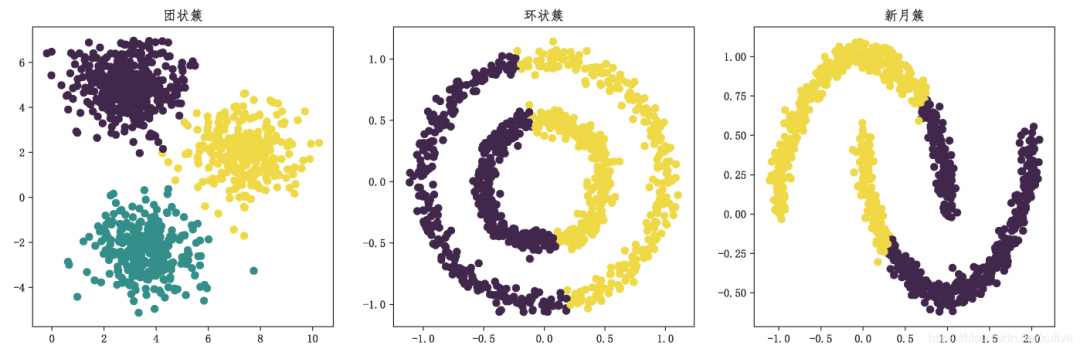
Centroid-based clustering, whether k-means clustering or mean shift clustering, has obvious limitations: it cannot handle irregular sample distributions such as elongated, circular, or intersecting shapes.
k-means clustering is usually regarded as the “entry-level algorithm” for clustering, and its algorithm principle is very simple. First, select k samples from the X dataset as centroids, and then repeat the following two steps to update the centroids until they no longer move significantly: the first step assigns each sample to the nearest centroid, and the second step creates new centroids based on the average of all samples for each centroid.
Centroid-based clustering gathers data by separating samples into multiple classes with the same variance, hence it always hopes that the clusters are convex and isotropic, but this is not always achievable. For example, for clusters with irregular shapes such as elongated, circular, or intersecting, the clustering effect is poor.
from sklearn import datasets as dss # Import sample generator
from sklearn.cluster import KMeans # Import clustering model from clustering submodule
import matplotlib.pyplot as plt
plt.rcParams['font.sans-serif'] = ['FangSong']
plt.rcParams['axes.unicode_minus'] = False
X_blob, y_blob = dss.make_blobs(n_samples=[300,400,300], n_features=2)
X_circle, y_circle = dss.make_circles(n_samples=1000, noise=0.05, factor=0.5)
X_moon, y_moon = dss.make_moons(n_samples=1000, noise=0.05)
y_blob_pred = KMeans(init='k-means++', n_clusters=3).fit_predict(X_blob)
y_circle_pred = KMeans(init='k-means++', n_clusters=2).fit_predict(X_circle)
y_moon_pred = KMeans(init='k-means++', n_clusters=2).fit_predict(X_moon)
plt.subplot(131)
plt.title('Blob Clusters')
plt.scatter(X_blob[:,0], X_blob[:,1], c=y_blob_pred)
plt.subplot(132)
plt.title('Circular Clusters')
plt.scatter(X_circle[:,0], X_circle[:,1], c=y_circle_pred)
plt.subplot(133)
plt.title('Moon Clusters')
plt.scatter(X_moon[:,0], X_moon[:,1], c=y_moon_pred)
plt.show()
The above code first uses a sample generator to generate blob clusters, circular clusters, and moon clusters, and then applies k-means clustering to each. The results indicate that k-means clustering is only suitable for blob clusters, while it fails for circular and moon clusters. The final clustering effects are shown in the figure below.
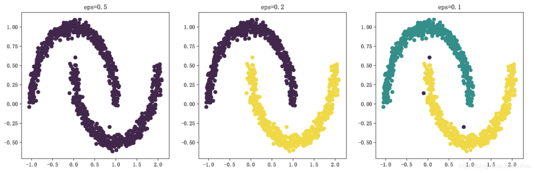
Density-based spatial clustering has better adaptability and can discover clusters of any shape.
Density-based spatial clustering, fully known as the density-based spatial clustering of applications with noise (DBSCAN), views clusters as high-density regions separated by low-density regions, which is completely different from the assumption of k-means clustering that clusters are always convex, thus allowing for the discovery of clusters of any shape.
The DBSCAN class is a density-based spatial clustering algorithm provided by the clustering submodule of Scikit-learn, which has two important parameters: eps and min_samples. To understand the parameters of the DBSCAN class, one must first understand core samples. If a sample has at least min_samples samples (including itself) within the eps distance range, it is called a core sample. Thus, the parameters eps and min_samples define the density of the cluster.
from sklearn import datasets as dss
from sklearn.cluster import DBSCAN
import matplotlib.pyplot as plt
plt.rcParams['font.sans-serif'] = ['FangSong']
plt.rcParams['axes.unicode_minus'] = False
X, y = dss.make_moons(n_samples=1000, noise=0.05)
dbs_1 = DBSCAN() # Default core sample radius 0.5, core sample neighbors 5
dbs_2 = DBSCAN(eps=0.2) # Core sample radius 0.2, core sample neighbors 5
dbs_3 = DBSCAN(eps=0.1) # Core sample radius 0.1, core sample neighbors 5
dbs_1.fit(X)
DBSCAN(algorithm='auto', eps=0.5, leaf_size=30, metric='euclidean', metric_params=None, min_samples=5, n_jobs=None, p=None)
dbs_2.fit(X)
DBSCAN(algorithm='auto', eps=0.2, leaf_size=30, metric='euclidean', metric_params=None, min_samples=5, n_jobs=None, p=None)
dbs_3.fit(X)
DBSCAN(algorithm='auto', eps=0.1, leaf_size=30, metric='euclidean', metric_params=None, min_samples=5, n_jobs=None, p=None)
plt.subplot(131)
plt.title('eps=0.5')
plt.scatter(X[:,0], X[:,1], c=dbs_1.labels_)
plt.subplot(132)
plt.title('eps=0.2')
plt.scatter(X[:,0], X[:,1], c=dbs_2.labels_)
plt.subplot(133)
plt.title('eps=0.1')
plt.scatter(X[:,0], X[:,1], c=dbs_3.labels_)
plt.show()
The above code uses DBSCAN with appropriate parameters to successfully separate the upper and lower moon datasets, with the results shown in the figure below.
Principal Component Analysis (PCA) is a statistical method and the most commonly used dimensionality reduction method.
PCA transforms a set of possibly correlated variables into a set of linearly uncorrelated variables through orthogonal transformation; the transformed variables are called principal components. Clearly, PCA’s dimensionality reduction is not simply discarding some features, but rather merging correlated high-dimensional variables into linearly independent low-dimensional variables through orthogonal transformation, thus achieving dimensionality reduction.
The following code demonstrates how to use the PCA class to perform principal component analysis and dimensionality reduction using the iris dataset. It is known that the iris dataset has 4 feature columns, namely the length and width of the sepals and the length and width of the petals.
from sklearn import datasets as dss
from sklearn.decomposition import PCA
ds = dss.load_iris()
ds.data.shape # 150 samples, 4 feature dimensions (150, 4)
m = PCA() # Instantiate PCA class with default parameters, n_components=None
m.fit(ds.data) # Fit the model
m.explained_variance_ # Variance values of each component after orthogonal transformation
array([4.22824171, 0.24267075, 0.0782095 , 0.02383509])
m.explained_variance_ratio_ # Proportion of variance values of each component to total variance
array([0.92461872, 0.05306648, 0.01710261, 0.00521218])
The results of the principal component analysis of the iris dataset show that there is one significant component whose variance value accounts for over 92% of the total variance; there is one component with a very small variance value, accounting for only 0.52% of the total variance; the first two components contribute over 97.7% of the variance, allowing the feature columns of the dataset to be reduced from 4 to 2 without losing too much effective information.
m = PCA(n_components=0.97)
m.fit(ds.data) # Fit the model
m.explained_variance_ # Variance values after orthogonal transformation
array([4.22824171, 0.24267075])
m.explained_variance_ratio_ # Proportion of variance values after orthogonal transformation
array([0.92461872, 0.05306648])
d = m.transform(ds.data) # Transform the dataset
d.shape(150, 2)
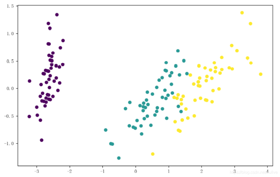
By specifying the parameter n_components to be at least 0.97, we can obtain the dimensionality reduction results of the original dataset: still 150 samples, but only 2 feature columns. If these 2 feature columns are viewed as x and y coordinates in a Cartesian coordinate system, all sample data can be intuitively plotted.
import matplotlib.pyplot as plt
plt.scatter(d[:,0], d[:,1], c=ds.target)
plt.show()
The figure below shows that using only 2 feature dimensions can still distinguish the 3 types of iris flowers.