This article uses a visual presentation to help you deeply understand the structure of the LSTM model.
Recently, I have been learning about the application of LSTM in time series prediction, but I encountered a significant problem: after adding time steps to the traditional BP network, its structure becomes difficult to understand.At the same time, the input and output data formats are also challenging to grasp. There are many articles online that introduce the structure of LSTM, but they are not intuitive and are very unfriendly to beginners. I also spent a long time pondering and looking at a lot of materials and shared LSTM structure diagrams from netizens to understand the intricacies.The content of this article is as follows:
1. Traditional BP Network and CNN Network
2. LSTM Network
3. LSTM Input Structure
4. LSTM in PyTorch
    4.1 LSTM Model Defined in PyTorch
    4.2 Data Format for LSTM
    4.3 LSTM Output Format
5. LSTM Combined with Other Networks
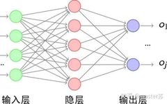
1. Traditional BP Network and CNN NetworkThe BP network and CNN network do not have a time dimension, and are quite similar to traditional machine learning algorithms. When CNN processes a color image with 3 channels, it can be understood as stacking multiple layers, and the three-dimensional matrix of the image can be understood as spatial slices. When writing code, just stack it layer by layer according to the diagram. The following images show a typical BP network and CNN network.
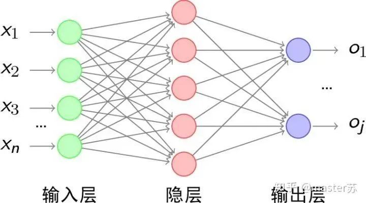 BP Network
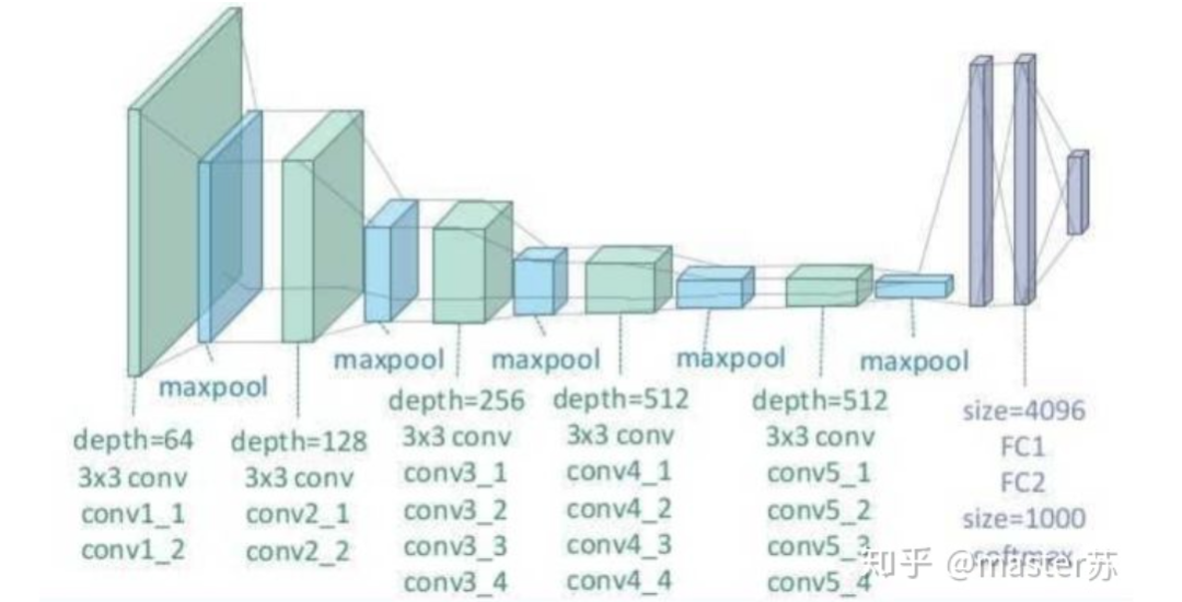 CNN NetworkThe hidden layers, convolutional layers, pooling layers, and fully connected layers in the diagram actually exist, and they are stacked layer by layer, which is easy to understand spatially. Therefore, when writing code, it is basically just looking at the diagram to write code, for example, using Keras:
# Example code, no practical significance
model = Sequential()
model.add(Conv2D(32, (3, 3), activation='relu'))  # Add convolutional layer
model.add(MaxPooling2D(pool_size=(2, 2)))         # Add pooling layer
model.add(Dropout(0.25))                          # Add dropout layer
model.add(Conv2D(32, (3, 3), activation='relu'))  # Add convolutional layer
model.add(MaxPooling2D(pool_size=(2, 2)))         # Add pooling layer
model.add(Dropout(0.25))                          # Add dropout layer
....   # Add other convolution operations
model.add(Flatten())                            # Flatten the three-dimensional array to two-dimensional array
model.add(Dense(256, activation='relu'))        # Add a normal fully connected layer
model.add(Dropout(0.5))
model.add(Dense(10, activation='softmax'))
....  # Train the network
2. LSTM NetworkWhen we search for the LSTM structure online, the most common image we see is the one below: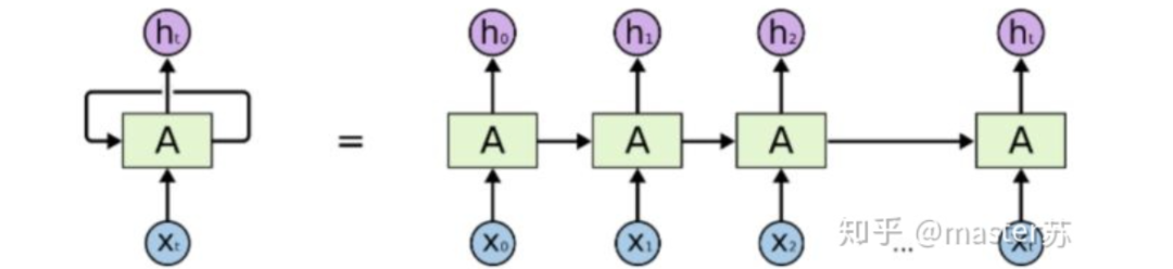 RNN NetworkThis is the classic structure diagram of the RNN recurrent neural network. LSTM only improves the hidden layer node A, while the overall structure remains unchanged. Therefore, this article also discusses the visualization of this structure.The middle A node hidden layer shows that the left side represents an LSTM network with only one hidden layer. The so-called LSTM recurrent neural network utilizes cycles on the time axis, and when expanded along the time axis, it produces the right diagram.Looking at the left diagram, many students mistakenly believe that LSTM is a single input, single output network structure with only one hidden neuron. Looking at the right diagram, they think that LSTM has multiple inputs and outputs, with multiple hidden neurons, where the number of A represents the number of hidden layer nodes.WTH? It’s hard to wrap my mind around this. This is the traditional network and spatial structure thinking.In fact, in the right diagram, we see Xt representing the sequence, where the subscript t is the time axis. Therefore, the number of A represents the length of the time axis, which is the state (Ht) of the same neuron at different times, not the number of hidden layer neurons.We know that the LSTM network uses the information from the previous moment, combined with the input information from the current moment, for training.For example, on the first day, I got sick (initial state H0), then took medicine (utilizing input information X1 to train the network), the next day I improved but wasn’t completely well (H1), took medicine again (X2), and my condition improved (H2), repeating until I recover. Therefore, the input Xt is taking medicine, the time axis T is the number of days of taking medicine, and the hidden layer state is my health condition. Thus, I am still me, just in different states.In fact, the LSTM network looks like this:
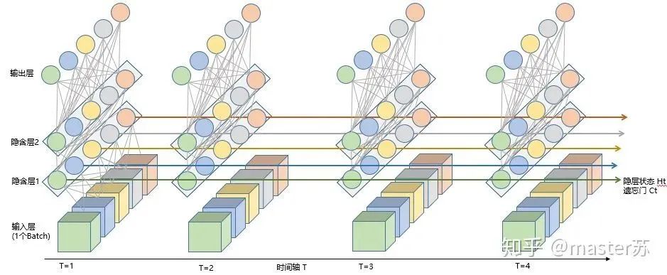 LSTM Network Structure
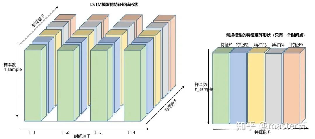
The above diagram represents an LSTM network with two hidden layers. When viewed at T=1, it is a normal BP network, and at T=2, it is also a normal BP network. However, when expanded along the time axis, the hidden layer information H and C trained at T=1 will be passed to the next moment T=2, as shown in the diagram below. The five arrows pointing to the right in the above diagram also indicate the transfer of hidden layer states along the time axis.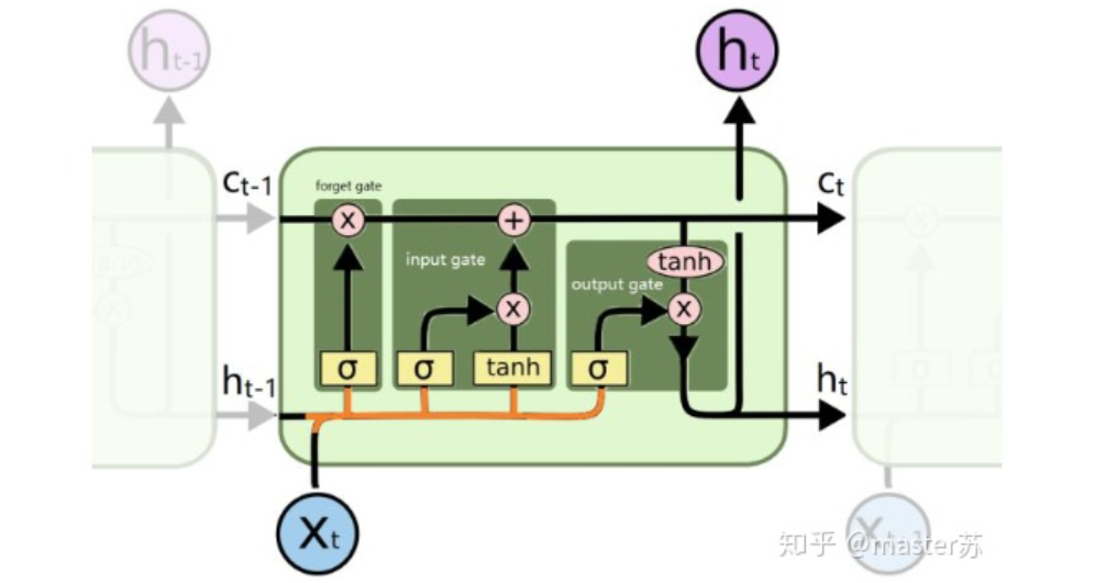 Note that in the diagram, H represents the hidden layer state, and C is the forget gate, which will be explained later regarding their dimensions.3. LSTM Input StructureTo better understand the LSTM structure, it is also essential to understand the data input situation of LSTM. Mimicking the appearance of a 3-channel image, the multi-sample, multi-feature data cube at different moments with the time axis is shown in the diagram below:
 Three-Dimensional Data Cube
The right diagram shows the input format we commonly see in models such as XGBOOST, LightGBM, decision trees, etc., where the input data format is a (N*F) matrix. The left side shows the data cube with the time axis added, which is a slice on the time axis, and its dimensions are (N*T*F), where the first dimension is the number of samples, the second dimension is time, and the third dimension is the number of features, as shown in the diagram below:

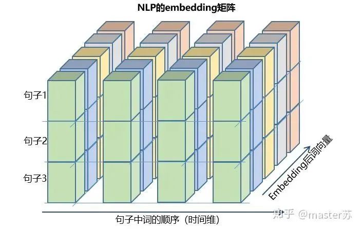
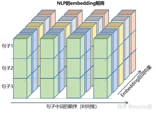
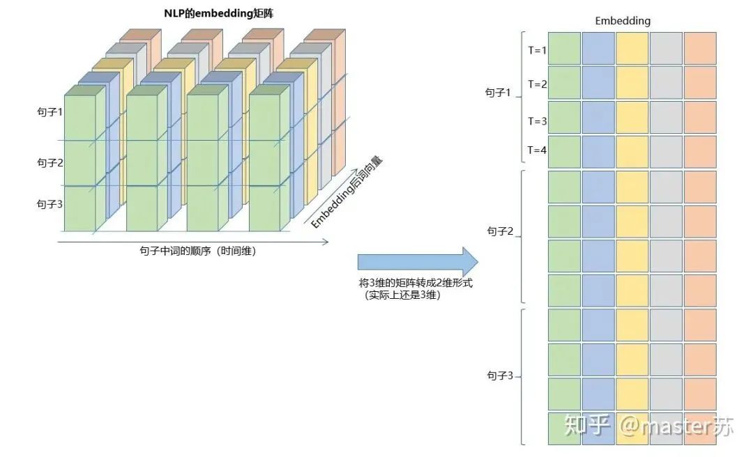
This kind of data cube is abundant, for example, in weather forecast data, samples can be understood as cities, the time axis as dates, and features as weather-related factors like rainfall, wind speed, PM2.5, etc. This data cube is easy to understand. In NLP, a sentence is embedded into a matrix, where the order of words is the time axis T, and the embedding of multiple sentences forms a three-dimensional matrix as shown in the diagram below:
4. LSTM in PyTorch
4.1 LSTM Model Defined in PyTorch
The parameters of the LSTM model defined in PyTorch are as follows:
class torch.nn.LSTM(*args, **kwargs)
Parameters are:
    input_size: dimension of x's features
    hidden_size: dimension of hidden layer's features
    num_layers: number of LSTM hidden layers, default is 1
    bias: False means bihbih=0 and bhhbhh=0. Default is True
    batch_first: True means the input/output data format is (batch, seq, feature)
    dropout: applies dropout to each layer's output except the last layer, default: 0
    bidirectional: True means bidirectional LSTM, default is False
Combining with the previous diagrams, let’s look at them one by one.(1) input_size:The dimension of x’s features, which is F in the data cube. In NLP, it is the length of the vector after a word is embedded, as shown in the diagram below: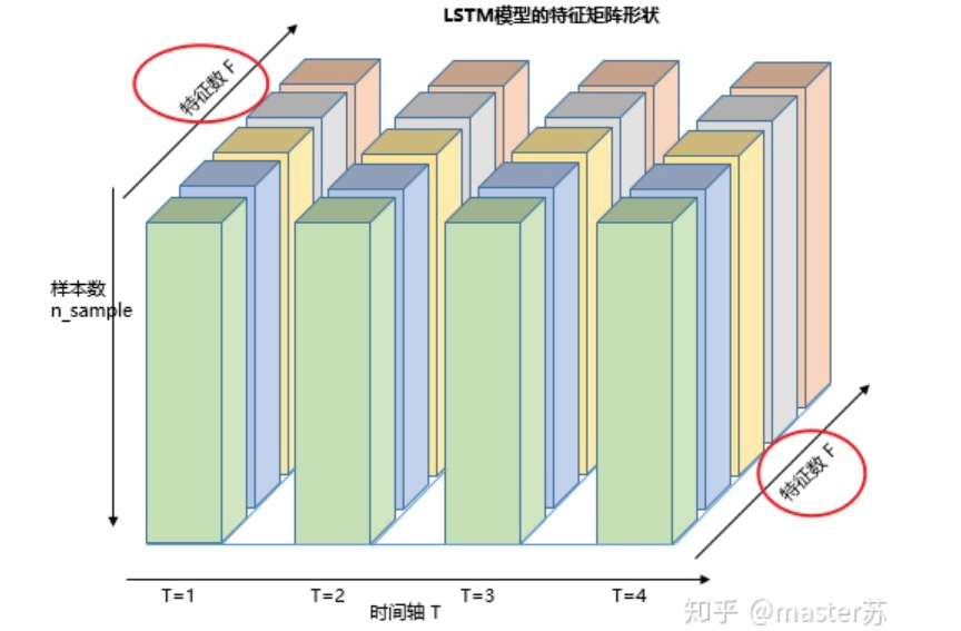 (2) hidden_size:The dimension of the hidden layer’s features (number of hidden layer neurons), as shown in the diagram below. We have two hidden layers, each with a feature dimension of 5. Note that the output dimension of a non-bidirectional LSTM equals the hidden layer’s feature dimension.
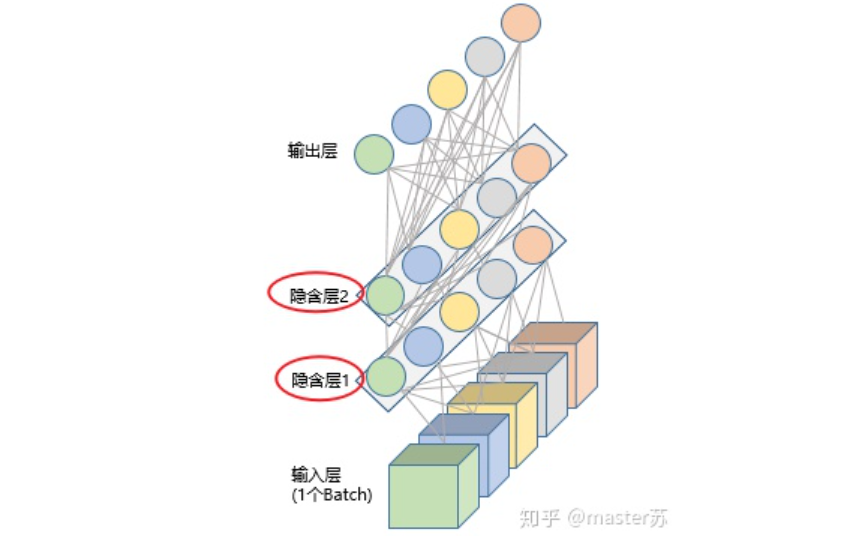 (3) num_layers:The number of LSTM hidden layers, as shown in the diagram above, where we defined 2 hidden layers.(4) batch_first:Used to define the input/output dimensions, which will be discussed later.(5) bidirectional:Whether it is a bidirectional recurrent neural network. The diagram below shows a bidirectional recurrent neural network. Therefore, when using a bidirectional LSTM, I need to pay special attention: during forward propagation, there are (Ht, Ct) and during backward propagation, there are also (Ht’, Ct’). Previously, we mentioned that the output dimension of a non-bidirectional LSTM equals the hidden layer’s feature dimension, while the output dimension of a bidirectional LSTM is the number of hidden layer features * 2, and the dimensions of H and C are the length of the time axis * 2.
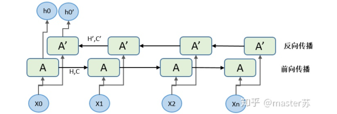
4.2 Data Format for LSTM
The default input data format for LSTM in PyTorch is as follows:
input(seq_len, batch, input_size)
Parameters are:
    seq_len: sequence length, in NLP it is the sentence length, generally padded using pad_sequence to match lengths
    batch: the number of data entries fed to the network at once, in NLP it is how many sentences are fed to the network at once
    input_size: feature dimension, consistent with the input_size defined in the network structure.
It was also mentioned earlier that if the LSTM parameter batch_first=True, then the required input format is:
input(batch, seq_len, input_size)Just swap the positions of the first two parameters. This is actually a relatively easy-to-understand data format. Below, I will explain how to construct the input for LSTM using embedding vectors in NLP.Previously, our embedding matrix looked like this:
If the batch is placed first, the three-dimensional matrix form is as follows:
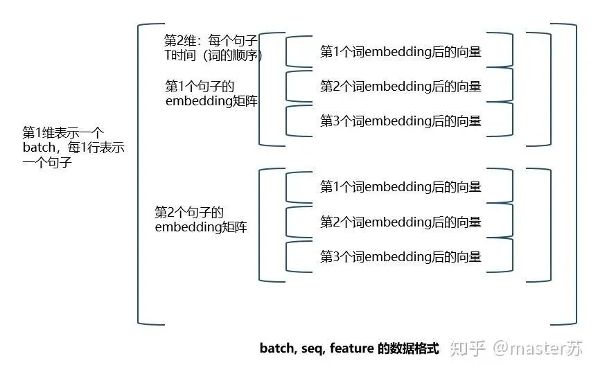
The transformation process is illustrated in the diagram below:
Did you understand? This is the input data format, isn’t it simple?The other two inputs for LSTM are h0 and c0, which can be understood as the network’s initialization parameters, generated using random numbers.
h0(num_layers * num_directions, batch, hidden_size)
c0(num_layers * num_directions, batch, hidden_size)
Parameters:
    num_layers: number of hidden layers
    num_directions: if it is a unidirectional recurrent network, then num_directions=1; if it is bidirectional, then num_directions=2
    batch: the input data batch
    hidden_size: number of hidden layer neurons
Note that if we define the input format as:
input(batch, seq_len, input_size)Then the formats of H and C must also change:
h0(batch, num_layers * num_directions, hidden_size)
c0(batch, num_layers * num_directions, hidden_size)
4.3 LSTM Output Format
The output of LSTM is a tuple as follows:
output,(ht, ct) = net(input)
    output: output of the hidden layer neurons at the last state
    ht: the hidden layer state value at the last state
    ct: the forget gate value at the last state
The default dimensions of output are:
output(seq_len, batch, hidden_size * num_directions)
ht(num_layers * num_directions, batch, hidden_size)
ct(num_layers * num_directions, batch, hidden_size)
Similar to the input situation, if we previously defined the input format as:
input(batch, seq_len, input_size)Then the formats of ht and ct must also change:
ht(batch, num_layers * num_directions, hidden_size)
ct(batch, num_layers * num_directions, hidden_size)
After all this, let’s go back and see where ht and ct are, please look at the diagram below: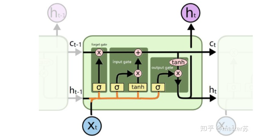 Where is the output? Please look at the diagram below:
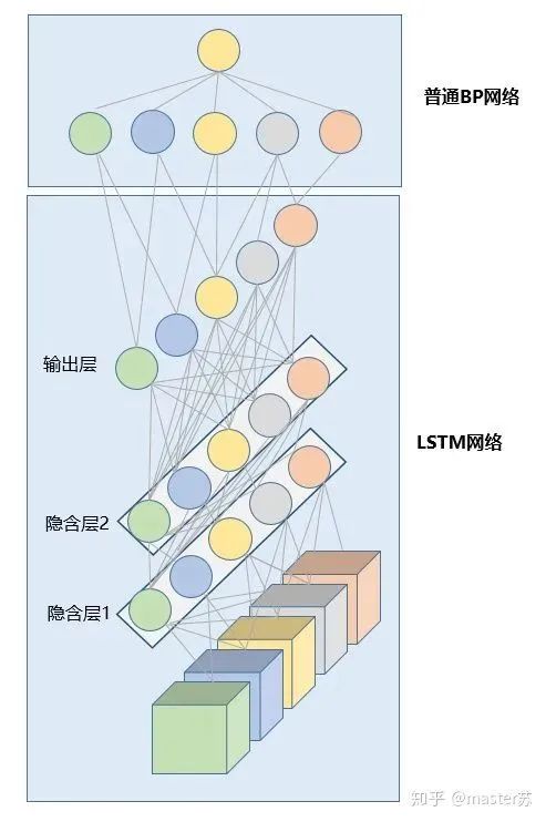
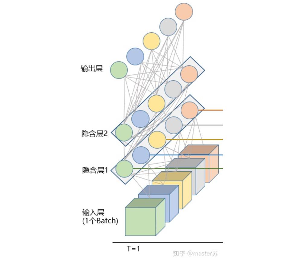 5. LSTM Combined with Other NetworksDo you remember that the dimension of output equals the number of hidden layer neurons, i.e., hidden_size? In some time series predictions, a fully connected layer is often added after the output, where the input dimension of the fully connected layer equals the LSTM’s hidden_size, and the subsequent network processing is the same as BP network, as shown in the diagram below:
 Using PyTorch to implement the above structure:
import torch
from torch import nn
class RegLSTM(nn.Module):
    def __init__(self):
        super(RegLSTM, self).__init__()
        # Define LSTM
        self.rnn = nn.LSTM(input_size, hidden_size, hidden_num_layers)
        # Define regression layer, input feature dimension equals LSTM output, output dimension is 1
        self.reg = nn.Sequential(
            nn.Linear(hidden_size, 1)
        )
    def forward(self, x):
        x, (ht, ct) = self.rnn(x)
        seq_len, batch_size, hidden_size = x.shape
        x = x.view(-1, hidden_size)
        x = self.reg(x)
        x = x.view(seq_len, batch_size, -1)
        return x
Of course, some models treat the output as the input for another LSTM or use the information from the hidden layers ht, ct for modeling; it varies.Alright, that’s my learning insights on LSTM. Remember to follow and like after reading.Reference links:https://zhuanlan.zhihu.com/p/94757947https://zhuanlan.zhihu.com/p/59862381https://zhuanlan.zhihu.com/p/36455374https://www.zhihu.com/question/41949741/answer/318771336https://blog.csdn.net/android_ruben/article/details/80206792Link:https://zhuanlan.zhihu.com/p/139617364This article is for academic exchange only. If there is any infringement, please contact us to delete it.