Using CorrGAN: Comparing Network-Based and Minimum Variance Portfolios

Star★TopPublic Account Love You All♥

Editor: 1+1=6

Introduction

Many econophysicists have noted that portfolios constructed using the empirical correlation matrix estimated from stock (or other asset) returns are very similar to those obtained from minimum variance optimization using the empirical covariance estimated for the same stocks.

The companies of the minimum risk Markowitz portfolio [MVP] are always located on the outer leaves of the [minimum spanning] tree. ——Onnela, J.-P., A. Chakraborti, K. Kaski, J. Kertész, and A. Kanto (2003). Dynamics of market correlations: Taxonomy and portfolio analysis. Phys. Rev. E 68(5), 056110*

This recurring fact (the similarity of the portfolios obtained from these two different methods) has led researchers to believe that there may be a profound mathematical connection between the two methods.

Huttner et al. pointed out in a very interesting paper that this is not the case:

Through Monte Carlo simulations, the authors show that generally, the solutions of the two portfolio construction methods are quite different: the minimum variance portfolio does not necessarily invest in the outer leaves of the network extracted from the same correlation matrix.

So, how can we explain the empirical fact that researchers are concerned about?

Huttner et al. believe it may arise from the special nature of the actual empirical correlation matrices (rather than the consistent random correlation matrices they used for Monte Carlo simulations).

They point out in the paper:

the previous Monte Carlo studies should be rerun using simulation algorithms that are able to produce correlation matrices that display only a subset of these stylized facts, as opposed to completely random correlation matrices (which display none of them) and market correlation matrices (which exhibit them all). […] Concerning the generation of correlation matrices whose MSTs exhibit the scale-free property, to the best of our knowledge there is no algorithm available, and due to the generating mechanism of the MST we expect the task of finding such correlation matrices to be highly complex.

We believe that GANs can provide useful insights into this problem:

• GANs can help sample real financial correlations (CorrGAN).

• Exploring their latent space can better understand the properties of financial correlation matrices.

• Hopefully, by separating the latent space, it will be easy to control the generative model and sample only correlation matrices, thus validating the issues raised by Huttner et al.

CorrGAN Paper Link: https://arxiv.org/pdf/1910.09504.pdf

Currently, we only sample from CorrGAN (a GAN based on thousands of correlation matrices estimated from the historical returns of S&P 500 stocks) and verify that the minimum variance portfolio indeed invests in the outer leaves of the network extracted from the same correlation matrix.

%matplotlib inline

import os
import numpy as np
import pandas as pd
import fastcluster
from scipy.cluster import hierarchy
from multiprocessing import Pool
from numpy.random import beta
from numpy.random import randn
from scipy.linalg import sqrtm
from numpy.random import seed
from tqdm import tqdm
import matplotlib.pyplot as plt


seed(42)

We define two functions:

• Calculate minimum variance weights
• Calculate eigenvector centrality (one of the definitions of network centrality)

The concept of centrality is often used in network analysis. Typically, there are two starting points for centrality analysis: degree and potential.

Degree indicates the extent to which a node is central in the network; potential indicates the closeness of the entire graph. In other words, degree reflects the properties of individual nodes, while potential reflects the properties of the entire graph.

Full Random Correlation Matrices Sampled Using the Onion Method

The onion method is a way to sample uniformly from the correlation matrix of a subset accurately.

The specific description of this method can be found in:

https://www.semanticscholar.org/paper/Behavior-of-the-NORTA-method-for-correlated-random-Ghosh-Henderson/d20f94efe7353594c804cc515e94817bd91b8f26

This sampling process may be interesting when studying the in-sample and out-of-sample behavior of some portfolio construction algorithms and how they compare with each other.

Onion Method:

import numpy as np
from numpy.random import beta
from numpy.random import randn
from scipy.linalg import sqrtm
from numpy.random import seed

seed(42)
def sample_unif_correlmat(dimension):
    d = dimension + 1

    prev_corr = np.matrix(np.ones(1))
    for k in range(2, d):
        # sample y = r^2 from a beta distribution with alpha_1 = (k-1)/2 and alpha_2 = (d-k)/2
        y = beta((k - 1) / 2, (d - k) / 2)
        r = np.sqrt(y)

        # sample a unit vector theta uniformly from the unit ball surface B^(k-1)
        v = randn(k-1)
        theta = v / np.linalg.norm(v)

        # set w = r theta
        w = np.dot(r, theta)

        # set q = prev_corr**(1/2) w
        q = np.dot(sqrtm(prev_corr), w)

        next_corr = np.zeros((k, k))
        next_corr[:(k-1), :(k-1)] = prev_corr
        next_corr[k-1, k-1] = 1
        next_corr[k-1, :(k-1)] = q
        next_corr[:(k-1), k-1] = q

        prev_corr = next_corr
        
    return next_corr
sample_unif_correlmat(3)
array([[ 1.        ,  0.36739638,  0.1083456 ],
       [ 0.36739638,  1.        , -0.05167306],
       [ 0.1083456 , -0.05167306,  1.        ]])
from mpl_toolkits.mplot3d import Axes3D
import matplotlib.pyplot as plt


fig = plt.figure()
ax = fig.add_subplot(111, projection='3d')

n = 1000

correlmats = [sample_unif_correlmat(3) for i in range(n)]
xs = [correlmat[0,1] for correlmat in correlmats]
ys = [correlmat[0,2] for correlmat in correlmats]
zs = [correlmat[1,2] for correlmat in correlmats]


for c, m, zlow, zhigh in [('r', 'o', -50, -25), ('b', 'o', -30, -5)]:
    ax.scatter(xs, ys, zs, c=c, marker=m)

ax.set_xlabel('$\rho_{12}$')
ax.set_ylabel('$\rho_{13}$')
ax.set_zlabel('$\rho_{23}$')

plt.show()

Code Display ↑↑↑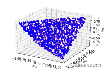

We can observe an elliptical shape, which is the collection of all correlation matrices. We can effectively sample uniformly from this collection!

The following function can be used to sample uniformly random correlation matrices on the elliptical cross-section according to the onion method.

def sample_unif_correlmat(dimension):
    d = dimension + 1

    prev_corr = np.matrix(np.ones(1))
    for k in range(2, d):
        # sample y = r^2 from a beta distribution
        # with alpha_1 = (k-1)/2 and alpha_2 = (d-k)/2
        y = beta((k - 1) / 2, (d - k) / 2)
        r = np.sqrt(y)

        # sample a unit vector theta uniformly
        # from the unit ball surface B^(k-1)
        v = randn(k-1)
        theta = v / np.linalg.norm(v)

        # set w = r theta
        w = np.dot(r, theta)

        # set q = prev_corr**(1/2) w
        q = np.dot(sqrtm(prev_corr), w)

        next_corr = np.zeros((k, k))
        next_corr[:(k-1), :(k-1)] = prev_corr
        next_corr[k-1, k-1] = 1
        next_corr[k-1, :(k-1)] = q
        next_corr[:(k-1), k-1] = q

        prev_corr = next_corr
        
    return prev_corr

Code Display ↑↑↑

Actual Financial Correlation Matrices Generated by CorrGAN

Load 10,000 correlation matrices of size 100 x 100 generated by CorrGAN.

n = 100
a, b = np.triu_indices(n, k=1)

gan_corrs = []
for r, d, files in os.walk('gan_corrs/'):
    for file in files:
        flat_corr = np.load('gan_corrs/{}'.format(file))
        corr = np.ones((n, n))
        corr[a, b] = flat_corr
        corr[b, a] = flat_corr
        gan_corrs.append(corr)
 
plt.figure(figsize=(5, 5))
plt.pcolormesh(gan_corrs[0])
plt.show()

Code Display ↑↑↑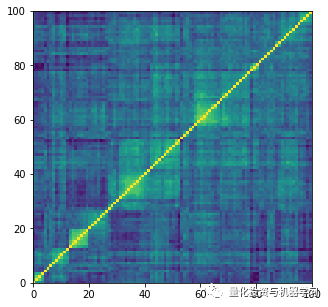

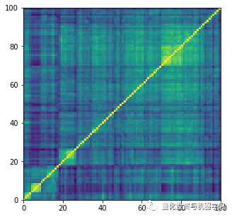
Empirical Correlation Matrices of S&P 500 Constituents

real_corrs = []
for r, d, files in os.walk('corrs_med/'):
    for file in files:
        if 'corr_emp_100d_batch' in file:
            flat_corr = pd.read_hdf('corrs_med/{}'.format(file))
            corr = np.ones((n, n))
            corr[a, b] = flat_corr
            corr[b, a] = flat_corr
            real_corrs.append(corr)
            
        if len(real_corrs) >= 10000:
            break
dist = 1 - real_corrs[0]
Z = fastcluster.linkage(dist[a, b], method='ward')
permutation = hierarchy.leaves_list(
    hierarchy.optimal_leaf_ordering(Z, dist[a, b]))
prows = real_corrs[0][permutation, :]
ordered_corr = prows[:, permutation]

plt.figure(figsize=(5, 5))
plt.pcolormesh(ordered_corr)
plt.show()

Code Display ↑↑↑

MVP and Eigenvector Centrality

The statistics defined below are used to measure the extent to which MVP invests in the outer leaves of the network:

(Portfolio weight over 20% of total assets) / 0.2

If, on average, this statistic equals 1, it means there is no relationship between MVP and eigenvector centrality. If significantly lower than 1, MVP will invest in central assets. If far greater than 1, then MVP will invest in leaves.

def compute_stat_1(C, p=0.2):
    MVP_weights = compute_mv_weights(C)
    centralities = compute_eigenvector_centrality(C)
    # find the k (20%) smallest values
    k = int(len(C) * p)
    idx = centralities.argsort()[:k]
    
    return MVP_weights[idx].sum() / p

Code Display ↑↑↑

Monte Carlo Simulation

nb_samples = len(gan_corrs)
list_nb_assets = [gan_corrs[0].shape[0]]

unif_ratios = {}
gan_ratios = {}
real_ratios = {}
for nb_assets in list_nb_assets:
    correlmats = [sample_unif_correlmat(nb_assets)
                  for sample in tqdm(range(nb_samples))]
    
    with Pool() as pool:
        values = list(
            tqdm(pool.imap_unordered(compute_stat_1,
                                     correlmats),
                 total=nb_samples))
        
unif_ratios[nb_assets] = values
    
    with Pool() as pool:
        values = list(
            tqdm(pool.imap_unordered(compute_stat_1,
                                     gan_corrs),
                 total=nb_samples))
        
gan_ratios[nb_assets] = values
    
    with Pool() as pool:
        values = list(
            tqdm(pool.imap_unordered(compute_stat_1,
                                     real_corrs),
                 total=nb_samples))
    
    real_ratios[nb_assets] = values

for d in list_nb_assets:
    unif_density, unif_edges, unif_hist = plt.hist(
        unif_ratios[d], bins=10000, density=True,
        stacked=True)
    unif_proba = sum([v for (v, b) in zip(unif_density, unif_edges)
                      if b <= 1]) * (unif_edges[1] - unif_edges[0])
    plt.clf()
    gan_density, gan_edges, gan_hist = plt.hist(
        gan_ratios[d], bins=10000, density=True,
        stacked=True)
    gan_proba = sum([v for (v, b) in zip(gan_density, gan_edges)
                     if b <= 1]) * (gan_edges[1] - gan_edges[0])
    plt.clf()
    real_density, real_edges, real_hist = plt.hist(
        real_ratios[d], bins=10000, density=True,
        stacked=True)
    real_proba = sum([v for (v, b) in zip(real_density, real_edges)
                      if b <= 1]) * (real_edges[1] - real_edges[0])
    plt.clf()
        
    plt.figure(figsize=(15, 10))
    plt.title(r'$rac{portfolio~weight~of~the~20	ext{%~least~central~assets}}{0.2}$'
              + "	for correlation matrices with shape $100 \times 100$",
              fontsize=16)
    bins = np.linspace(-6, 20, 100)
    
    # uniform random correlation matrices
    plt.hist(unif_ratios[d], bins, alpha=0.8,
             label="(unif correl mats) mean = "
             + str(round(np.mean(unif_ratios[d]), 2))
             + ", proba(stat < 1) = " + str(round(np.mean(unif_proba), 2)))
    plt.axvline(x=np.mean(unif_ratios[d]),
                color='b', linestyle='dashed', linewidth=2)
    
    # real financial correlation matrices
    plt.hist(real_ratios[d], bins, alpha=0.8,
             label="(real correl mats) mean = "
             + str(round(np.mean(real_ratios[d]), 2))
             + ", proba(stat < 1) = " + str(round(np.mean(real_proba), 2)))
    plt.axvline(x=np.mean(real_ratios[d]),
                color='r', linestyle='dashed', linewidth=2)
    
    # realistic random correlation matrices generated by CorrGAN
    plt.hist(gan_ratios[d], bins, alpha=0.8,
             label="(gan correl mats) mean = "
             + str(round(np.mean(gan_ratios[d]), 2))
             + ", proba(stat < 1) = " + str(round(np.mean(gan_proba), 2)))
    plt.axvline(x=np.mean(gan_ratios[d]),
                color='g', linestyle='dashed', linewidth=2)
    
    # baseline: 1 means no relation between centrality and MV weights
    plt.axvline(x=1, color='k', linestyle='dashed', linewidth=2)
    
    plt.legend()
    plt.show()

Code Display ↑↑↑

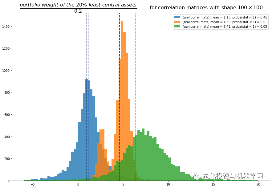
We can use consistent random correlation matrices to reproduce Huttner et al.’s conclusions: generally, the minimum variance group investments have no relationship with centrality (blue distribution).

However, for the market return estimates of actual correlation matrices (orange distribution), we can note that the mean of the statistics is significantly greater than 1, and even stronger, with no values below 1. This confirms the empirical researchers’ view: Markowitz/Minimum Variance Portfolios (MVPs) tend to invest in the leaves of the correlated network. All MVP portfolios constructed based on actual correlations tend to be biased towards assets located at the edge of the network. Why is the statistical distribution bimodal? Is it because there are essentially two types of correlation matrices and MVPs? For example, a comparison between stressed market periods and normal market periods. During periods of high correlation under stress, the correlation network will take on a star topology (assuming one central asset and many leaves directly connected to this central asset). In this initial configuration, many leaves will receive approximately equal allocations, so the 20% least central assets will not exceed the baseline of 20%. However, under normal circumstances, risk factors are more diversified to drive assets, and the correlation/network topology will contain deeper and fewer correlated leaves, which will receive more allocation from the MVP, hence weights exceeding the baseline allocation of 20%. This hypothesis requires further research.

Regarding the correlation matrices generated by CorrGAN, the authors also show that for actual financial correlations, MVPs and network-based portfolios tend to select the same assets. Only 5% of portfolios do not exceed 20% core assets. However, besides this, these 20% least central assets even have larger weights than those using actual empirical correlation matrices. We can see that GANs do not fully capture all the properties of empirical matrices: when we use synthetic matrices, the statistics used to compare MVPs and network-based portfolios do not exhibit a bimodal distribution.