Click the above“Visual Learning for Beginners”, select to add “Star” or “Pin”
Important content delivered promptly
With the emergence of social networking services like Facebook and Instagram, the volume of image data generated has seen a tremendous increase over the past decade. The use of image (and video) processing software such as GNU Gimp and Adobe Photoshop to create modified images and videos is a primary concern for internet companies like Facebook.
These images are a major source of fake news and are often used maliciously to incite riots. Before taking action on suspicious images, we must verify their authenticity. The IEEE Information Forensics and Security Technical Committee (IFS-TC) initiated a detection and localization forensics challenge, the first image forensics challenge in 2013, to address this issue. They provided an open digital image dataset that includes images captured under different lighting conditions, as well as forged images generated using the following algorithms:
-
Content-aware filling and patch matching (for copy/paste)
-
Content-aware repair (for copy/paste and stitching)
-
Clone stamp (copy/paste)
-
Seam carving (image retargeting)
-
Inpainting (reconstruction of damaged parts of an image – a special case of copy/paste)
-
Alpha matting (for stitching)
Two Phases of the Challenge
The first phase requires participating teams to classify images as forged or original (not manipulated).
The second phase requires them to detect/localize the forged regions in the forged images.
Why Use CNN?
In the era before deep learning in artificial intelligence, image processing researchers designed handcrafted features to tackle general image processing problems, particularly image classification problems. One such example is the Sobel kernel used for edge detection. The previously used image forensics tools can be categorized into five types:
-
Pixel-based techniques that detect statistical anomalies introduced at the pixel level.
-
Format-based techniques that exploit statistical correlations introduced by specific lossy compression schemes.
-
Camera-based techniques that exploit artifacts introduced by camera lenses, sensors, or chip post-processing.
-
Physics-based techniques that explicitly model and detect anomalies in the three-dimensional interactions between physical objects, light, and cameras.
-
Geometry-based techniques that measure objects in the world and their positions relative to the camera.
Almost all of these techniques utilize content-based features of the image, i.e., the visual information presented in the image. CNNs are inspired by the visual cortex. Technically, these networks are designed to extract features that are meaningful for classification, i.e., those features that minimize the loss function. By using gradient descent to learn network parameters – kernel weights, they generate the most distinctive features from the images fed to the network. These features are then provided to a fully connected layer that performs the final classification task.
After observing several forged images, it became apparent that the human visual cortex can detect forged areas. Thus, CNNs are the perfect deep learning model for this task. If the human visual cortex can detect it, then this network designed specifically for the task will surely be more powerful.
Dataset
Before diving into the dataset overview, it is essential to clarify the terms used:
-
Forged images: Images that have been processed/manipulated using the two most common operations, namely copy/paste and image stitching.
-
Original images: Images that have not been manipulated, except for resizing all images to standard dimensions according to competition rules.
-
Image stitching: The stitching operation can combine human images, add doors to buildings, trees to parking lots, cars, etc. Stitched images may also contain parts produced by copy/paste operations. The image receiving the stitched parts is referred to as the “host” image. The parts stitched together with the host image are called “aliens”.
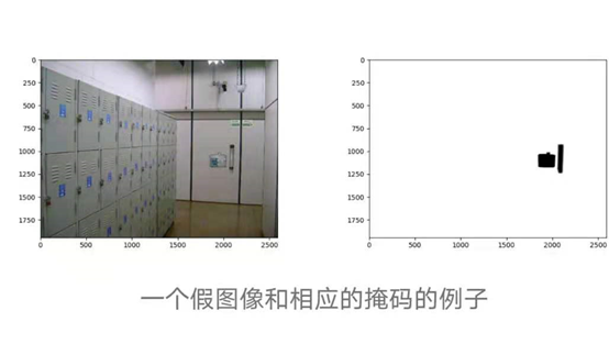
The entire dataset for the first and second phases can be found here. For this project, we will only use the training set. It contains two directories – one with fake images and their corresponding masks, and another with original images. The masks for the fake images are black and white (non-gray) images that describe the stitched regions of the fake images. The black pixels in the mask indicate the areas where operations were performed on the source image to obtain the forged image, specifically the stitched regions.
This dataset consists of 1050 original images and 450 forged images.Color images typically have three channels, one each for red, green, and blue, but sometimes a fourth yellow channel may appear.Images in our dataset are a mix of 1, 3, and 4-channel images.After observing some 1-channel images, i.e., grayscale images.
The challenge organizers intentionally added these images as they wanted to address such noise. Although some blue images could be images of clear skies. Therefore, some were included while others were discarded as noise. Take a look at four-channel images – they also contain no useful information. They are merely pixel grids filled with 0 values. Thus, the cleaned original dataset contains approximately 1025 RGB images.
The forged images are a mix of 3 and 4-channel images, but none are noise. The corresponding masks are a mix of 1, 3, and 4-channel images. The feature extraction we will use only needs to retrieve information from one channel of the mask. Therefore, our forged image corpus consists of 450 fakes. Next, we performed a train-test split to retain 20% for the final test from the 1475 images.
Feature Extraction from the Training Set
The current state of the dataset is not suitable for training a model. It must be transformed into a state that is very suitable for the task at hand, namely detecting anomalies introduced by forging operations at the pixel level. With this in mind, we designed the following method to create relevant images from the given data.
For each fake image, we have a corresponding mask. We use this mask to sample the fake image along the boundaries of the stitched regions to ensure that both the forged and unforge parts of the image contribute at least 25%. These samples will have distinctive boundaries that only appear in the fake image. These boundaries will be learned by our designed CNN. Since the three channels of the mask contain the same information (the forged parts of the image at different pixels), we only need one channel to extract samples.
To make the boundaries of the images clearer, the grayscale images are first converted to binary images through thresholding (implemented with OpenCV), followed by Gaussian filtering for denoising. After this operation, sampling is done by moving a 64×64 window (8 steps) across the fake image, counting the 0-value (black) pixels in the corresponding mask if the value is sampled within a certain interval.
In [29]:# Convert grayscale images to binarybinaries=[]

for grayscale in x_train_masks:    blur = cv2.GaussianBlur(grayscale,(5,5),0)    ret,th = cv2.threshold(blur,0,255,cv2.THRESH_BINARY+cv2.THRESH_OTSU)    binaries.append(th)In [56]:~binaries[28]Out[56]:array([[0, 0, 0, ..., 0, 0, 0],       [0, 0, 0, ..., 0, 0, 0],       [0, 0, 0, ..., 0, 0, 0],       ...,       [0, 0, 0, ..., 0, 0, 0],       [0, 0, 0, ..., 0, 0, 0],       [0, 0, 0, ..., 0, 0, 0]], dtype=uint8)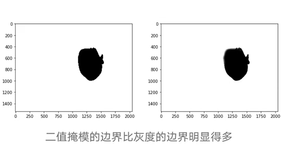
After sampling, we obtained 175,119 64×64 patches from the fake images. To generate 0-labeled (original) patches, we sampled approximately the same number from the real images. Finally, we have 350,728 patches, which are divided into multiple sequences and cross-validation sets.
Now we have a large high-quality input image dataset. It is time to experiment with various CNN architectures.
Custom CNN Architecture
The first architecture we tried was inspired by the original architectural research papers. Their input image size was 128×128×3, thus the network was large. Since we have half the spatial size, our network is also smaller. This is the architecture we attempted first.
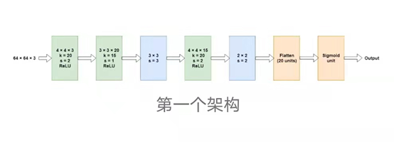
The green layers are convolutional, and the blue ones are Max pooling. The network was trained on 150,000 sample columns (for testing) and 25,000 validation samples. The network has 8536 parameters, which is relatively few compared to the training samples, thus avoiding the need for more aggressive dropout. A dropout rate of 0.2 was applied to the flattened output of 20 units. We used the default learning rate (0.001) and the Adam optimizer with beta_1 and beta_2. After approximately ___ epochs, the results were as follows:
Training accuracy: 77.13%, Training loss: 0.4678
Validation accuracy: 75.68%, Validation loss: 0.5121
These numbers are not very impressive, as in 2012, CNNs overwhelmingly beat expert-engineered feature programs developed over years of research. However, considering that we did not use any image forensics knowledge (pixel statistics and related concepts) to achieve an accuracy of ___ on unseen data, these numbers are not too bad either.
Transfer Learning
Since this is a CNN that has beaten all classical machine learning algorithms on the ImageNet classification task, why not leverage the work of one of these powerful machines to tackle the problem at hand? This is the idea behind transfer learning. In short, we use the weights of a pre-trained model to solve our problem, a model that may have been trained on a larger dataset and yielded better results when addressing its problem. In other words, we “transfer” the learning of one model to our own model. In our case, we used VGG16 trained on the ImageNet dataset to vectorize the images in our dataset. Here, we tried two approaches:
-
Using the bottleneck features outputted by VGG16 and building a shallow network on top of it.
-
Fine-tuning the last convolutional layer of the VGG16+Shallow model from (1).
Intuitively, (2) yielded much better results than (1). We tried various shallow network architectures and eventually arrived at this:
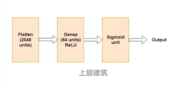
The input to the flattened layer is the bottleneck features outputted by VGG16. These are tensors of shape (2×2×512) since we used 64×64 input images.
The architecture above yielded the following results:
Training accuracy: 83.18%, Training loss: 0.3230
Validation accuracy: 84.26%, Validation loss: 0.3833
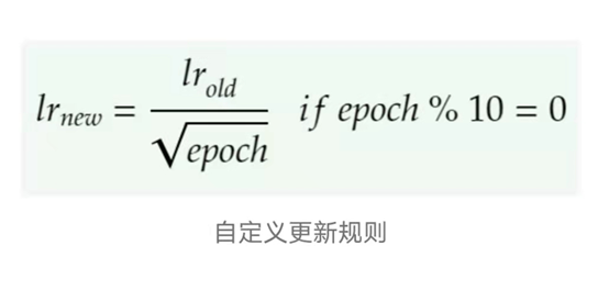
We trained using the Adam optimizer, with a custom learning rate that decreases every 10 epochs (in addition to being regularly updated by Adam after each batch).
The second method required fine-tuning the last layer. An important point to note here is that for fine-tuning, we must use a pre-trained top model. The goal is to slightly change the weights that have already been mastered to better fit the data. If we use some randomly initialized weights, slight changes will not benefit them, while large changes will destroy the learned weights of the convolutional layers. We also need a very small learning rate to fine-tune our model (for the same reasons mentioned above). After this, it is recommended to use the SGD optimizer for fine-tuning. However, we observed that Adam performed better on this task than SGD.
The fine-tuned model yielded the following results:
Training accuracy: 99.16%, Training loss: 0.018
Validation accuracy: 94.77%, Validation loss: 0.30
The slightly overfitted model can be remedied by using a smaller learning rate (we used 1e-6).
Besides VGG16, we also tried ResNet50 and VGG19 models with pre-trained bottleneck features on the ImageNet dataset. The features from ResNet50 performed better than VGG16. VGG19’s performance was not very satisfactory. We fine-tuned the ResNet50 architecture (last convolutional layer) in a similar manner to VGG16, using the same learning rate update strategy, yielding more promising results with smaller overfitting issues.
Training accuracy: 98.65%, Training loss: 0.048
Validation accuracy: 95.22%, Validation loss: 0.18
Final Model Prediction on Test Data
To sample images from the previously created test set, we adopted a strategy similar to that used to create the training and cross-validation sets, i.e., using the mask to sample fake images at the boundaries and sampling the same number of original images of the same size. We used the fine-tuned VGG16 model to predict the labels of these patches, yielding the following results:
Test accuracy: 94.65%, Test loss: 0.31
On the other hand, ResNet50 yielded the following results on the test data:
Test accuracy: 95.09%, Test loss: 0.19
As we can see, our model performed very well. We still have plenty of room for improvement. If more data can be generated through data augmentation (cropping, resizing, rotating, and other operations), perhaps we can fine-tune more SOTA network layers.
Download 1: OpenCV-Contrib Extension Module Chinese TutorialReply in the background of the “Visual Learning for Beginners” official account:Extension Module Chinese Tutorial, to download the first OpenCV extension module tutorial in Chinese available online, covering installation of extension modules, SFM algorithms, stereo vision, object tracking, biological vision, super-resolution processing, and more than twenty chapters of content.Download 2: Python Vision Practical Projects 52 LecturesReply in the background of the “Visual Learning for Beginners” official account: Python Vision Practical Projects, to download 31 visual practical projects including image segmentation, mask detection, lane line detection, vehicle counting, eyeliner addition, license plate recognition, character recognition, emotion detection, text content extraction, facial recognition, etc., to aid in the rapid learning of computer vision.Download 3: OpenCV Practical Projects 20 LecturesReply in the background of the “Visual Learning for Beginners” official account: OpenCV Practical Projects 20 Lectures, to download 20 practical projects based on OpenCV to advance OpenCV learning.
Discussion Group
Welcome to join the reader group of the official account to communicate with peers. Currently, there are WeChat groups for SLAM, three-dimensional vision, sensors, autonomous driving, computational photography, detection, segmentation, recognition, medical imaging, GAN, algorithm competitions, etc. (these will gradually be subdivided), please scan the WeChat ID below to join the group, and note: “nickname + school/company + research direction”, for example: “Zhang San + Shanghai Jiao Tong University + Visual SLAM”. Please follow the format for notes, otherwise, your request will not be approved. Once successfully added, you will be invited into the relevant WeChat group based on your research direction. Please do not send advertisements in the group, otherwise you will be removed, thank you for understanding~