Understanding the Technological Foundation of AI: Vector Databases

// Introduction

As we know, we are deeply caught in the whirlpool of an artificial intelligence (AI) revolution. No matter which industry AI intervenes in, it brings revolutionary hopes and possibilities, while also triggering brand new challenges. For applications including large language models, generative AI, and semantic search, how to effectively handle data has become particularly important.

The foundation of most innovative applications based on large language models is built on the so-called “vector embedding” technology, which is a data representation method containing key semantic information that helps AI systems understand and store long-term memories to accomplish complex tasks.

Vector embeddings can be generated by AI models (such as large language models) and contain a large number of attributes or features. This makes managing their representations challenging. In the fields of AI and machine learning, these features represent various dimensions of data, which are crucial for understanding patterns, relationships, and potential structures.

That’s why we need a database specifically designed to handle such data. Vector databases provide optimized storage and querying capabilities for embeddings, thus meeting this demand.

Relational databases and non-relational databases are both systems used for storing and querying data, but they differ significantly in terms of data organization, performance, scalability, and use cases. Here’s a detailed introduction to both:

Relational Databases: Relational databases (RDBMS) are based on the “relational model,” storing data in predefined tables, with relationships established between tables through foreign keys. Each table consists of rows and columns, where each column contains specific attributes for each entry in the table, and each row represents a record. RDBMS can ensure data consistency, atomicity, isolation, and durability (the ACID properties). Examples include MySQL, Oracle, and SQL Server.

Non-relational Databases: Non-relational databases (NoSQL) do not rely on traditional table structures to store data, but instead use various data models such as key-value pairs, column families, documents, and graphs. This gives non-relational databases advantages in handling large amounts of dispersed data, parallel computation, and highly variable data structures. For example:

• Vector Databases: Vector databases are a type of non-relational database specifically designed to store and process vector data. These databases are mainly used for applications that require an understanding of the intrinsic semantics of data (e.g., using deep learning and AI technologies). Vector databases are designed to handle high-dimensional data and can efficiently perform similarity searches and other vector-related queries.

• Graph Databases: Graph databases use graph structures to store data, where nodes represent entities and edges represent relationships between entities. They outperform relational databases and other non-relational databases when data and relationships are complex and highly interconnected. Examples include Neo4j and Amazon Neptune.

• Document Stores: Document databases store data in the form of documents, typically in JSON or XML format. Each document can contain a set of key-value pairs, which can be nested and include complex data types. Document databases are very flexible and can easily handle irregular or dynamic data structures. Common document databases include MongoDB and CouchDB.

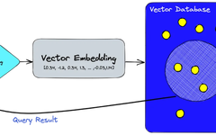
A typical application framework based on vector databases can be represented as follows:

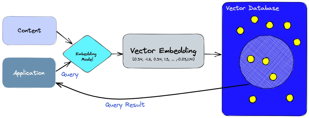
Breaking it down, it can be divided into several steps:

• First, we use an embedding model to create vector embeddings for the content we want to index.

• Insert the vector embeddings into the vector database, referencing the original content that created the embeddings.

• When an application issues a query request, we use the same embedding model to create embeddings for the query and use these embeddings to query similar vector embeddings in the database.

Layman’s Version:

Suppose you run an online music platform and you want to recommend the songs that best match each user’s musical taste through AI algorithms. To achieve this, you first need to convert each song and the user’s musical taste into a vector. This vector may contain various characteristics of the song, such as rhythm, pitch, song type, etc., while for the user, it may include the types of songs they have listened to before, rated songs, and other information. These vectors are called embeddings, which compress complex song information or user information into a multi-dimensional vector that mathematically expresses the relationship between songs or users.

Then, you can insert these song embeddings into the vector database. When a user logs into the platform, we can query in the vector database based on their musical taste vector to find the closest song vectors to recommend these songs to the user.

This example does not utilize an embedding model; in practical applications, the process of vectorizing songs and users typically involves an embedding model that can convert entities (such as songs or users) with rich semantic information into vectors. For instance, you can use some embedding model to generate an embedding (which is a vector) for each song. This embedding can capture various characteristics of the song (such as genre, rhythm, lyrical sentiment, etc.). Similarly, you can generate user embeddings based on their listening history, ratings, preferred song types, etc.

In simple terms, a vector index can be seen as a component or core part of a vector database. The vector index focuses on query efficiency, while the vector database provides a complete solution for the storage and retrieval of vector data.

In the era of big data, independent vector indexes like Facebook AI Similarity Search (FAISS) have gained widespread use, excelling in enhancing the search and retrieval capabilities of vector embeddings. However, these standalone tools lack some key functionalities compared to databases. To address this shortcoming, vector databases have emerged, specifically designed for managing vector embeddings, offering multiple advantages over using vector indexes alone:

Data Management: Vector databases have user-friendly data storage functions such as inserting, deleting, and updating data, making the management and maintenance of vector data simpler than using standalone vector indexes like FAISS, which require additional integration of storage solutions, increasing complexity.

Metadata Storage and Filtering: Vector databases can store metadata associated with each vector entry, allowing users to perform more refined queries using metadata filters.

Scalability: Vector databases are designed to accommodate the need for scaling as data volumes and user demands grow, better supporting distributed and parallel processing. In contrast, achieving similar scalability with independent vector indexes may require custom solutions, such as deploying and managing them on Kubernetes clusters or other similar systems.

Real-time Updates: Vector databases typically support real-time data updates to adapt to dynamically changing data needs, while independent vector indexes may require a comprehensive re-indexing process when accepting new data, which is time-consuming and resource-intensive.

Backup and Collection: Vector databases can handle routine backup operations for all data stored in the database.

Integration with Ecosystems: Vector databases can be more easily integrated with other parts of the data processing ecosystem, such as ETL pipelines (like Spark), analytical tools (like Tableau and Segment), and visualization platforms (like Grafana). This integration simplifies data management processes and facilitates integration with AI-related tools like LangChain, LlamaIndex, and ChatGPT plugins.

Data Security and Access Control: Vector databases often come equipped with built-in data security features and access control mechanisms to protect sensitive information, which may not be achievable with standalone vector index solutions.

In summary, vector databases provide superior solutions for handling vector embeddings by addressing the limitations of independent vector indexes—such as scalability challenges, cumbersome integration processes, lack of real-time updates, and built-in security measures—ensuring a more effective and seamless data management experience.

For most of us, the operation of traditional databases is familiar—they store strings, numbers, and other types of scalar data in rows and columns. However, vector databases work with vectors, so their optimization and querying methods are quite different.

In traditional databases, we usually look for rows in the database that match the query exactly. In vector databases, we use similarity measures to find vectors that are most similar to the query.

Vector databases utilize various algorithms to implement approximate nearest neighbor (ANN) searches, including hashing, quantization, or graph-based searches, to optimize the search process.

These algorithms are integrated into a process to quickly and accurately find the neighbors of the query vector. Given that vector databases provide approximate results, we need to balance precision and speed. The more precise the result, the slower the query speed. However, a good system can provide a lightning-fast search experience while achieving near-perfect accuracy. Below is a common workflow for vector databases:

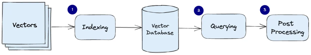
• Indexing: Vector databases use algorithms like PQ, LSH, or HNSW to index vectors. This step maps the vectors into a data structure to accelerate searches.

• Querying: The vector database compares the indexed query vector with indexed vectors in the dataset to find the nearest neighbors (using the similarity measure applied by the index).

• Post-processing: In some cases, the vector database retrieves the final nearest neighbors from the dataset and performs post-processing to return the final results. This step may involve re-sorting the nearest neighbors using different similarity measures.

In the following sections, we will delve deeper into these algorithms and explain how they collectively enhance the overall performance of vector databases.

Text Embedding

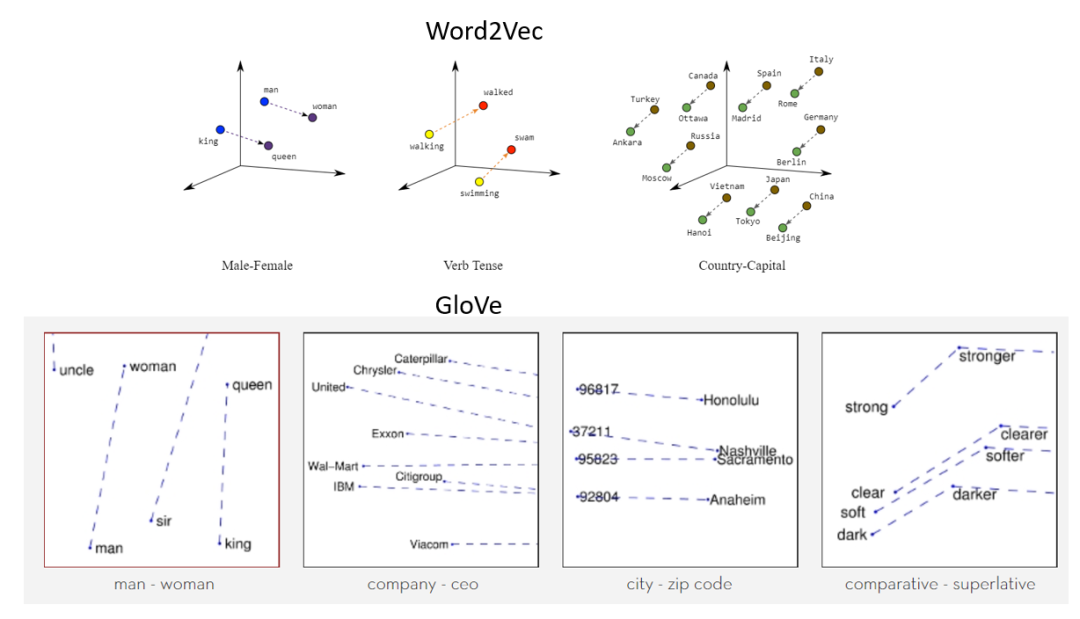
Text embedding techniques are primarily used to convert text data into a form that machine learning models can understand and use. Word2Vec, GloVe, and FastText are common word embedding techniques that map words to dense vectors. These techniques have wide applications in tasks such as text classification, sentiment analysis, and machine translation. Word2Vec has two architectures: Continuous Bag of Words (CBOW) and Skip-gram. GloVe learns word vectors by constructing a global word-word co-occurrence matrix. FastText builds on Word2Vec by incorporating character-level n-grams, making it advantageous in handling rare words and word forms. However, embeddings generated by these models often lack semantic context for words in specific contexts. To address this issue, researchers have introduced transformer-based models like BERT, GPT, and XLNet. These models can generate embeddings with more contextual semantics. Such models are typically pre-trained on large text datasets and can be fine-tuned for specific tasks.

Image Embedding

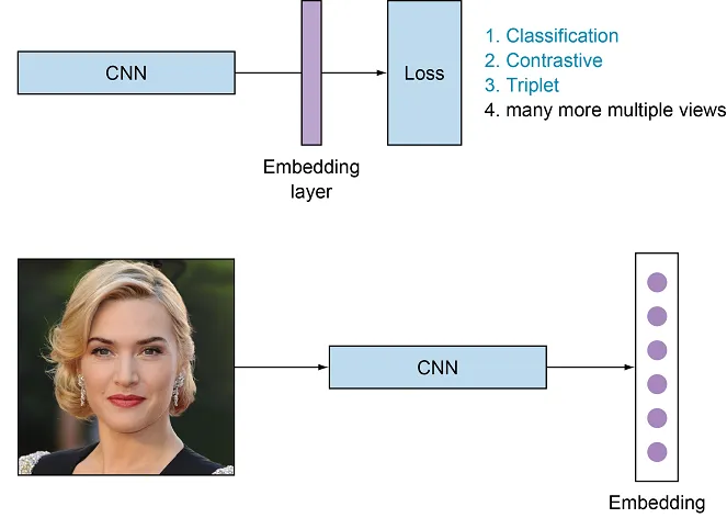
Image embedding techniques aim to convert image data into a form usable by machine learning models. Convolutional Neural Networks (CNNs) are the primary tools for image embedding, with architectures like VGG, ResNet, and Inception being classic models. These models extract local features of images through convolutional and pooling layers, generating high-dimensional vectors that represent the content of the images. In recent years, deep generative models such as Variational Autoencoders (VAEs) and Generative Adversarial Networks (GANs) have also been used to generate embedding vectors for images. Additionally, transformer models like ViT (Vision Transformer) have shown promise in image processing. ViT is a model that segments images into smaller patches and processes them using transformers.

Graph Embedding

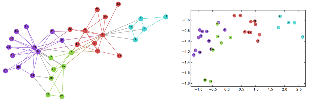
Graph embedding techniques aim to convert nodes and edges in a graph into a form usable by machine learning models. Classic algorithms such as DeepWalk and node2vec use random walks and the Word2Vec idea to generate embedding vectors for nodes in a graph. The GraphSAGE algorithm can generate embedding vectors for neighboring nodes. Graph Neural Networks (GNNs) and their variants such as GCN and GAT use node features and adjacency matrices to generate embeddings for nodes, demonstrating good performance in handling graph-structured data. These models can capture the topological structure of graphs and attribute information of nodes, encoding this information into low-dimensional vectors for subsequent tasks like node classification, link prediction, and graph classification.

Audio Embedding

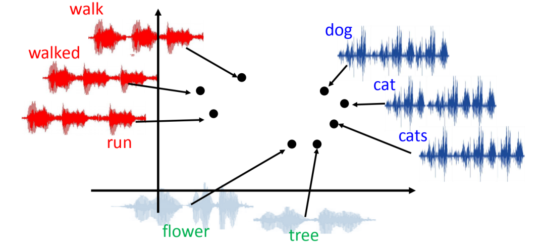
Audio embedding techniques aim to convert raw audio signals into a form understandable by machine learning models. Classic methods primarily use signal processing techniques such as Fourier Transform and MFCC (Mel-frequency cepstral coefficients) to extract audio features. Deep learning methods like Convolutional Neural Networks (CNNs) and Recurrent Neural Networks (RNNs) have widespread applications in audio embedding. For example, WaveNet is a generative model that can directly model raw audio waveforms. Recently, researchers have begun to explore using transformer models to process audio data, indicating the strong potential of transformer models for various types of data embeddings.

The core idea of most vector indexing algorithms is to compress vectors (fancy dimensionality reduction) to improve retrieval efficiency.

Random Projection

The basic idea behind random projection is to use a random projection matrix to project high-dimensional vectors into a lower-dimensional space. We create a random matrix whose size will be the target low-dimensional value we want. Then, we calculate the dot product of the input vector and the matrix to obtain a projection matrix with a lower dimension than our original vector while still retaining its similarity.

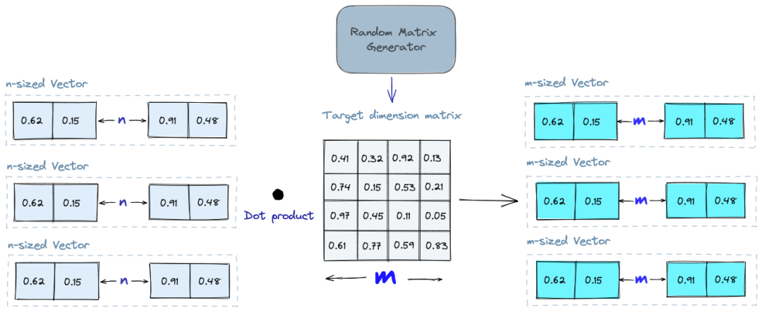
When we query, we project the query vector into the lower-dimensional space using the same projection matrix. We then compare the projected query vector with the projected vectors in the database to find the nearest neighbors. Because the dimensionality of the data is reduced, the search process is much faster than searching the entire high-dimensional space.

It’s important to remember that random projection is an approximate method, and the quality of the projection depends on the properties of the projection matrix. In general, the more random the projection matrix, the better the quality of the projection. However, generating truly random projection matrices can be computationally expensive, especially for large datasets.

Product Quantization

Another way to build an index is through product quantization (PQ), which is a lossy compression technique for high-dimensional vectors (such as vector embeddings). It takes the original vector, breaks it into smaller chunks, simplifies each chunk’s representation by creating a representative “code” for each chunk, and then recombines all the chunks together—without losing critical information essential for similarity operations. The PQ process can be divided into four steps: splitting, training, encoding, and querying.

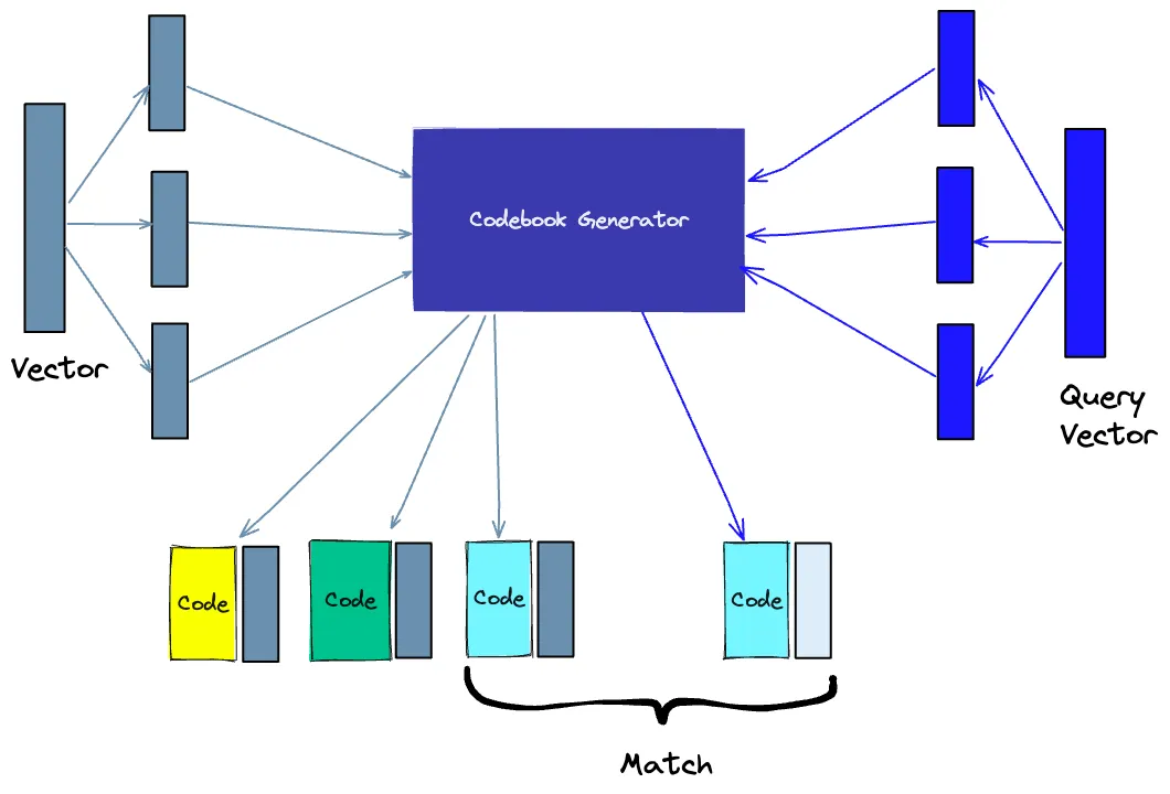
• Splitting – Decomposing the vector into segments.

• Training – We establish a “codebook” for each segment. Simply put, the algorithm generates a set of potential “codes” that may be assigned to the vector. In practice, this “codebook” consists of cluster centers generated by performing k-means clustering on each segment of the vectors. The number of values in the segment codebook will match the value we used for k-means clustering.

• Encoding – The algorithm assigns a specific code to each segment. In practice, after training is complete, we find the closest values in the codebook to each segment of the vector. Our PQ code will be identifiers of the corresponding values in the codebook. We can use as many PQ codes as possible, meaning we can select multiple values from the codebook to represent each segment.

• Querying – When we query, the algorithm decomposes the vector into subvectors and quantizes them using the same codebook. It then uses the indexed codes to find the vectors closest to the query vector.

The number of representative vectors in the codebook is a trade-off between representation accuracy and the computational cost of searching the codebook. The more representative vectors in the codebook, the more accurate the representation of vectors in the subspace, but the higher the computational cost of searching the codebook. Conversely, fewer representative vectors in the codebook lead to less accurate representation but lower computational costs.

Locality Sensitive Hashing

Locality Sensitive Hashing (LSH) is a technique used for indexing in approximate nearest neighbor searches. It optimizes speed while still providing approximate, non-exhaustive results. LSH uses a set of hash functions to map similar vectors into “buckets.”

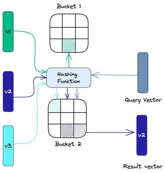
To find the nearest neighbors for a given query vector, we use the same hash functions as those for the “buckets” of similar vectors. The query vector is hashed into a specific table, and then compared with other vectors in the same table to find the closest match. This method is much faster than searching the entire dataset because the number of vectors in each hash table is far less than in the entire space.

It’s crucial to remember that LSH is an approximate method, and the quality of the approximation depends on the properties of the hash functions used. Generally, the more hash functions used, the better the quality of the approximation. However, using a large number of hash functions can be computationally expensive and may not be suitable for large datasets.

Hierarchical Navigable Small World (HNSW)

HNSW creates a hierarchical tree structure where each node represents a set of vectors. The edges between nodes represent the similarity between the vectors. The algorithm first creates a set of nodes, each containing a small number of vectors. This can be done randomly or by clustering the vectors using algorithms like k-means, with each cluster becoming a node.

Then, the algorithm examines the vectors of each node and draws edges between the node and the most similar vectors. When we query an HNSW index, it uses this graph to navigate through the tree, accessing the nodes that are most likely to contain the vectors closest to the query vector.

Vector of Local Aggregation Descriptor (VLAD)

VLAD is a technique used for aggregating feature descriptors, commonly applied in image and video retrieval tasks. The basic idea of VLAD is to aggregate a set of local descriptors (such as SIFT or SURF features) into a single vector descriptor that captures the statistical information within the set.

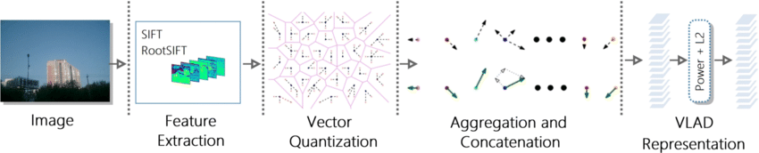
Here are the basic steps of VLAD:

1. First, train a Bag of Words (BoW) model consisting of k words (where words are points in vector space). This is usually achieved by clustering the descriptors from the training set using k-means.

2. For the set of descriptors to be encoded, each descriptor is assigned to the nearest word in the BoW model.

3. Then, for each word, compute the sum of the residuals (differences) of all descriptors assigned to that word. The result is a descriptor with the same dimension as the original descriptor.

4. The descriptors for all words are concatenated to form a large vector whose dimension is the product of the original descriptor dimension and the number of words.

5. This vector is often further processed, such as l2 normalization, to enhance retrieval performance.

Based on the previously discussed algorithms, we need to understand the role of similarity measures in vector databases. These measures form the basis for vector databases to compare and identify the most relevant results for a given query. Similarity measures are mathematical methods used to determine the degree of similarity between two vectors in vector space. Vector databases use similarity measures to compare vectors stored in the database and identify the vectors that are most similar to a given query vector. Various similarity measures can be used, including:

• Cosine Similarity: Measures the cosine of the angle between two vectors in vector space. Its range is -1 to 1, where 1 represents identical vectors, 0 represents orthogonal vectors, and -1 represents opposite vectors.

• Euclidean Distance: Measures the straight-line distance between two vectors in vector space. Its range is 0 to infinity, where 0 represents identical vectors, and larger values represent increasingly dissimilar vectors.

• Dot Product: Measures the product of the magnitudes of two vectors and the cosine of the angle between them. Its range is -∞ to ∞, where positive values indicate vectors pointing in the same direction, 0 represents orthogonal vectors, and negative values indicate vectors pointing in opposite directions.

Choosing which similarity measure to use will affect the results obtained from the vector database. Each similarity measure has its own advantages and disadvantages, so it is crucial to select the appropriate measure based on use cases and requirements.

Each vector stored in the database contains metadata (metadata, also known as “data about data” or “data on top of data,” is data that describes other data. It provides detailed information about the data, such as its source, creation time, last modified time, size, format, owner, location, etc. Metadata can help us understand the meaning, use, and organization of data so that we can better manage and utilize it. For example, consider an audio file. The audio data (such as sound waves) itself is data, while the file’s name, creation date, duration, file size, encoding format, bitrate, etc., are metadata.). In addition to querying similar vectors, vector databases can also filter results based on metadata queries. To achieve this, vector databases typically maintain two indexes: one for vectors and one for metadata. Metadata filtering can occur either before or after the vector search itself, but in either case, there are challenges that can slow down the query process.

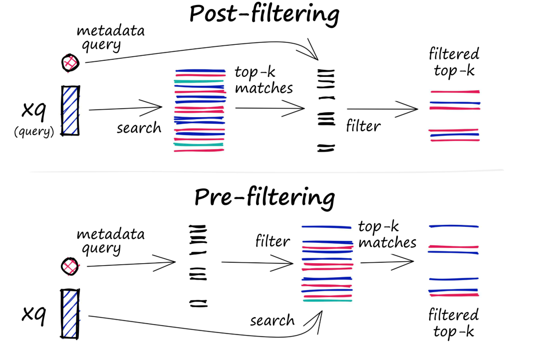
The filtering process can occur either before or after the vector search itself, but each method has its own challenges that may affect query performance:

• Pre-filtering: In this approach, metadata filtering occurs before vector search. While this can help reduce the search space, it may also cause the system to overlook relevant results that do not meet the metadata filtering criteria. Additionally, extensive metadata filtering may slow down the query process due to increased computational overhead.

• Post-filtering: In this approach, metadata filtering occurs after vector search. This ensures that all relevant results are considered, but it may also introduce additional overhead, requiring the system to filter out irrelevant results after the search is completed, which can slow down the query process.

To optimize the filtering process, vector databases employ various techniques, such as leveraging advanced indexing methods for metadata processing or using parallel processing to accelerate filtering tasks. Balancing trade-offs between search performance and filtering accuracy is crucial for providing efficient and relevant query results in vector databases.

Performance and Fault Tolerance

Performance and fault tolerance are two interrelated concepts. As the amount of data in our hands increases, the number of nodes required also increases, leading to a higher likelihood of errors and failures. Just as we expect from other types of databases, we want to be able to execute queries quickly even when some underlying nodes fail, whether such failures are due to hardware issues, network problems, or other types of technical issues. These failures may lead to system downtime or erroneous query results. To achieve high performance and high fault tolerance, vector databases adopt strategies of sharding and replication:

• Sharding: This method distributes data across multiple nodes. There are various ways to partition data; for example, it can be partitioned based on data similarity, allowing similar vectors to be stored in the same partition. During a query, the query request is sent to all shards, and results are retrieved and aggregated, known as the “scatter-gather” pattern.

• Replication: This method creates copies of data across different nodes. Thus, even if one node fails, other nodes can take over. Regarding replication, there are two main consistency models: eventual consistency and strong consistency. Eventual consistency allows temporary inconsistencies between data copies, enhancing availability and reducing latency, but may lead to data conflicts or even data loss. Strong consistency requires all data copies to be updated before a write operation is considered complete, providing stronger consistency but potentially leading to higher latency.

Monitoring

To effectively manage and maintain vector databases, we need a robust monitoring system to track the performance, health, and overall status of the database. Monitoring systems are crucial for identifying potential issues, optimizing performance, and ensuring smooth production operations. Typically, monitoring for vector databases focuses on the following aspects:

• Resource Usage: Monitoring resource usage, such as CPU, memory, disk space, and network activity, can help identify potential issues or resource constraints that may affect database performance.

• Query Performance: Query latency, throughput, and error rates may indicate system issues that require our attention and resolution.

• System Health: Overall system health monitoring includes the status of individual nodes, replication processes, and the status of other critical components.

Access Control

Access control is the process of managing and adjusting user access to data and resources, a key component of ensuring data security. It ensures that only authorized users can view, modify, or interact with sensitive data stored in the vector database. The importance of access control is highlighted in several ways:

• Data Protection: AI applications often need to handle sensitive and confidential information, and implementing stringent access control policies helps prevent unauthorized access and data breaches.

• Compliance: Many industries, such as healthcare and finance, are subject to strict data privacy regulations. Implementing appropriate access control can help organizations comply with these regulations, avoiding legal and financial issues.

• Accountability and Auditing: Access control mechanisms enable organizations to log user activities within the vector database. This information is crucial for auditing, assisting in tracking any unauthorized access or modifications when security breaches occur.

• Scalability and Flexibility: As organizations grow and evolve, access control needs may change. A robust access control system can seamlessly modify and scale user permissions, ensuring data security is maintained throughout the organization’s growth.

Backup and Collection

When all other protective measures fail, vector databases offer backup capabilities to regularly create copies of data. These backups can be stored in external storage systems or cloud services to ensure data security and recoverability. If data is lost or corrupted, these backups can be used to restore the database to a previous state, minimizing downtime and impact on the system.

APIs and SDKs

This is where the action happens: developers want easy-to-use, powerful APIs and SDKs for integrating and operating vector databases. A good API should be intuitive, easy to use, and have clear documentation, enabling developers to quickly understand and utilize it. On the other hand, SDKs should be compatible with mainstream programming languages and development environments.

References: https://www.pinecone.io/