Understanding Stable Diffusion: A Comprehensive Guide

Source: AI Algorithms and Image Processing


This article is about 4300 words, recommended reading time is 8 minutes.
A detailed interpretation of the stable diffusion paper, you will understand it after reading this article!

1. Introduction (Can Be Skipped)

Hello, everyone! I am Tian-Feng. Today, I will introduce some principles of stable diffusion in an easy-to-understand way. Since I usually play with AI drawing, I thought it would be nice to write an article explaining its principles. It took me a long time to write this article, and if you find it useful, I hope you can give it a thumbs up. Thank you.

Stable diffusion, as an open-source image generation model from Stability-AI, is on par with ChatGPT. Its development momentum is not inferior to Midjourney, and with the support of numerous plugins, its launch has been greatly enhanced. Of course, the techniques involved are slightly more complex than Midjourney.

As for why it’s open-source, the founder said: The reason I do this is that I believe it is part of a shared narrative. Some people need to publicly demonstrate what has happened. I want to emphasize again that this should be open-source by default. Because the value does not exist in any proprietary model or data, we will build auditable open-source models, even if they contain licensed data. Without further ado, let’s get started.

2. Stable Diffusion

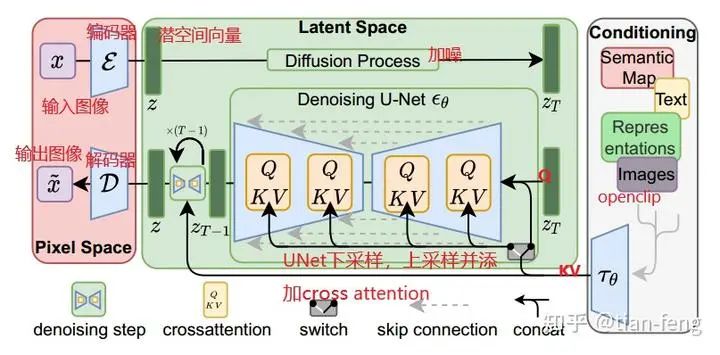
For the image in the original paper above, it may be difficult for some friends to understand, but it doesn’t matter. I will break down the image into individual modules for interpretation, and then combine them together. I believe you will understand what each step of the image does.

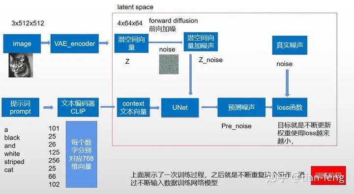
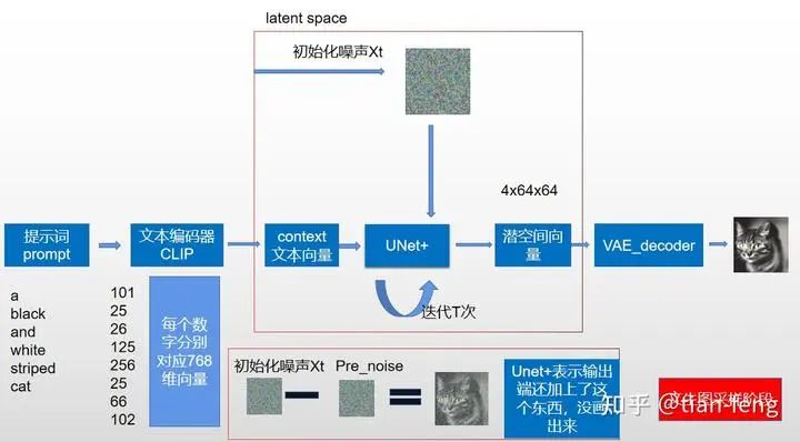
First, I will draw a simplified model diagram corresponding to the original image for easier understanding. Let’s start from the training phase. You may notice that the VAE decoder is missing. This is because our training process is completed in the latent space, and we will discuss the decoder in the second phase of sampling. The stable diffusion web UI we typically use for drawing usually operates in the sampling stage. As for the training phase, most ordinary people cannot achieve it. The training time required can be measured in GPU years (one V100 GPU takes about a year). If you have 100 GPUs, it should take about a month to complete. As for ChatGPT, the electricity costs are in the tens of millions of dollars, with thousands of GPU clusters. It seems that the current race in AI is about computing power. I digress, let’s come back.

1. CLIP

Let’s start with the prompt. When we input a prompt like ‘a black and white striped cat’, CLIP will map the text to a vocabulary where each word and punctuation mark corresponds to a number. We call each word a token. Previously, stable diffusion had a limit of 75 words for input (which is no longer the case), meaning 75 tokens. You may notice that 6 words correspond to 8 tokens because it also includes a start token and an end token. Each number corresponds to a 768-dimensional vector, which you can think of as the ID card of each word. Moreover, words with very similar meanings correspond to similar 768-dimensional vectors. After processing through CLIP, we obtain a (8,768) vector corresponding to the image’s text.

The stable diffusion uses the pre-trained model of OpenAI’s CLIP, which means we use a model that has already been trained. How is CLIP trained? How does it correspond images and text information? (The following is optional and does not affect understanding; just know that it is used to convert prompts into corresponding generated image text vectors.)

CLIP requires data consisting of images and their titles. The dataset contains about 400 million images and their descriptions. It should be obtained through web scraping, where the image information serves as labels. The training process is as follows:

CLIP is a combination of an image encoder and a text encoder, using two encoders to encode the data separately. Then, cosine distance is used to compare the resulting embeddings. Initially, even if the text description matches the image, their similarity is very low.

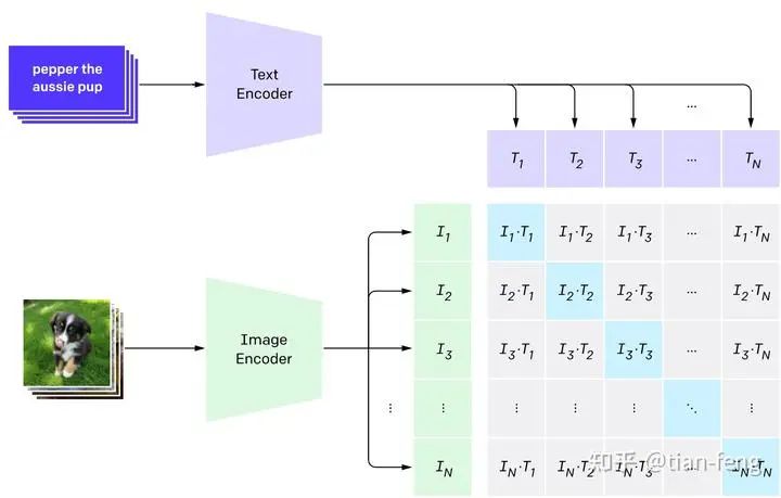
As the model continues to update, in subsequent phases, the embeddings obtained from encoding images and text will gradually become similar. This process is repeated across the entire dataset using a large batch size, ultimately generating an embedding vector where images of dogs and the phrase ‘a picture of a dog’ are similar.

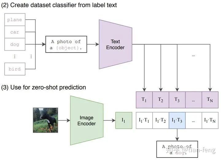
We provide some prompt texts, and for each prompt, we calculate similarity to find the one with the highest probability.

2. Diffusion Model

Now that we have an input for the UNet, we also need an input noise image. Suppose we input a 3x512x512 cat image; instead of directly processing the cat image, we compress the 512×512 image from pixel space to latent space (4x64x64) using a VAE encoder, reducing the data volume by nearly 64 times.

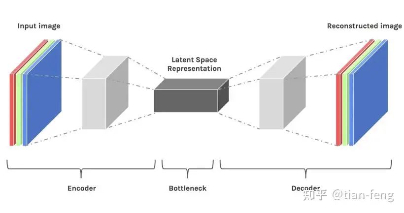
The latent space is simply a representation of compressed data. Compression refers to the process of encoding information using fewer bits than the original representation. Dimensionality reduction may lose some information; however, in some cases, reducing dimensions is not a bad thing. By reducing dimensions, we can filter out less important information and retain only the most significant information.

After obtaining the latent space vector, we now arrive at the diffusion model. Why can an image be restored after adding noise? The secret lies in the formulas. Here, I will explain the theory using the DDPM paper as a reference. Of course, there are also improved versions like DDIM, etc. If you’re interested, you can check them out yourself.

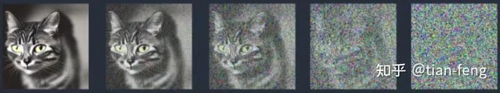
Forward Diffusion

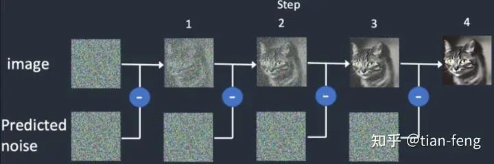
• First is forward diffusion, which is the noise addition process. Eventually, it turns into pure noise.

• At each moment, Gaussian noise must be added, and the next moment is obtained by adding noise to the previous moment.

So, do we need to obtain the noise at each step from the previous step? Can we obtain the noise image at any step we want? The answer is YES. This is because the noise we add during training is random. Suppose we randomly reach 100 steps of noise (assuming we set the total time steps to 200). If we want to add noise from the first step to get to the second step, it would be too time-consuming to loop back and forth. In fact, the added noise follows a pattern. Our goal now is to obtain the noisy image at any moment as long as we have the original image X0, without having to derive the desired noisy image step by step.

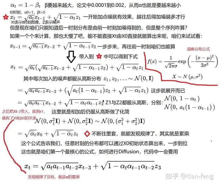
I will explain the above. I have marked everything clearly.

First, the range for αt is 0.9999-0.998.

Second, the noise added to the image follows a Gaussian distribution, meaning that the noise added to the latent space vector conforms to a mean of 0 and a variance of 1. By substituting Xt-1 into Xt, we can merge the two terms because Z1 and Z2 both follow a Gaussian distribution. Therefore, their sum Z2′ also follows a Gaussian distribution, and their variances sum to form a new variance. Thus, we sum their individual variances (the one with the square root is the standard deviation). If you cannot understand, you can treat it as a theorem. To elaborate, if Z–>a+bZ, then the Gaussian distributions of Z change from (0,σ) to (a,bσ). Now we have established the relationship between Xt and Xt-2.

Third, if you substitute Xt-2, you will get the relationship with Xt-3, and by finding the pattern, you will realize it is the cumulative product of α, and finally obtain the relationship between Xt and X0. Now we can directly obtain the noisy image at any moment based on this formula.

Fourth, since the initialization noise of the image is random, if you set the total time steps (timesteps) to 200, it means dividing the interval from 0.9999 to 0.998 into 200 parts, representing the α value at each moment. Based on the formula of Xt and X0, because of the cumulative product of α (which gets smaller), it can be seen that the noise increases faster as time progresses, roughly in the range of 1-0.13. At time 0, α is 1, which means Xt represents the image itself, while at time 200, the image has approximately α of 0.13, indicating that noise occupies 0.87 of it. Since it is cumulative, the noise increases, and it is not an average process.

Fifth, a quick note on the reparameterization trick.

If X(u,σ2), then X can be expressed as X=μ+σZ, where Z~Ν(0,1). This is the reparameterization trick.

The reparameterization trick allows sampling from a distribution that has parameters. If you sample directly (the sampling action is discrete and non-differentiable), there is no gradient information, and therefore, during backpropagation, the parameter gradients will not be updated. The reparameterization trick ensures that we can sample while retaining gradient information.

Reverse Diffusion

• After forward diffusion is completed, we move on to reverse diffusion, which might be more challenging. How do we obtain the original image from a noisy image step by step? This is the key.

• Reverse starts with our goal of obtaining the noise image Xt to get the noise-free X0. We begin from Xt to find Xt-1. Here, we first assume that X0 is known (we will ignore why we assume it is known for now). Later, we will replace it. As for how to replace it, we know the relationship between Xt and X0 from forward diffusion. Now we know Xt, we can express X0 in terms of Xt, but there is still an unknown noise Z at this point, which is where UNet comes into play. It needs to predict the noise.

• Here, we use Bayes’ theorem (which is conditional probability). We refer to the results of Bayes’ theorem; I previously wrote a document (https://tianfeng.space/279.html)

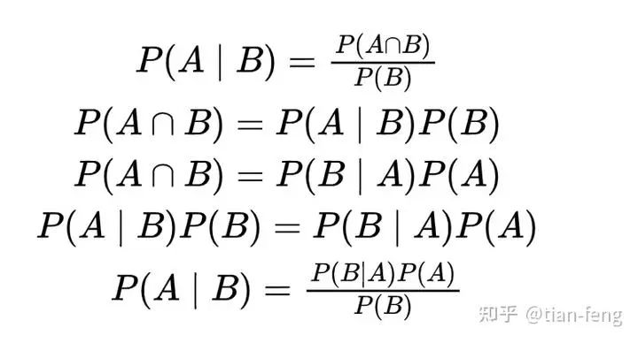
We start with known Xt to find Xt-1. In reverse, we don’t know how to find it, but we know how to find it forward. If we know X0, we can derive all these terms.

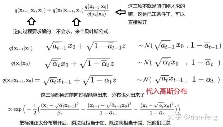
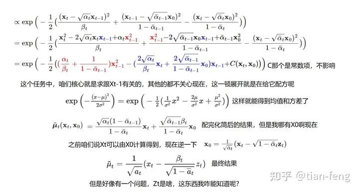
Let’s break it down. Since these three terms follow Gaussian distributions, substituting into the Gaussian distribution (also called normal distribution), why does their multiplication equal their sum? Because e2 * e3 = e2+3, which is understandable (it’s exp, meaning e raised to a power). Now we have obtained an overall equation, and we can continue simplifying:

First, we expand the square, and the unknown now is Xt-1, arranging it into the format AX2+BX+C. Don’t forget, even when added, they still follow Gaussian distributions. Now we align the original Gaussian distribution formula with the same format; the red part is the reciprocal of the variance, and the blue part multiplied by the variance divided by 2 gives us the mean μ (the result of simplification is shown below; if you’re interested, you can simplify it yourself). Returning to X0, we previously assumed X0 is known, now we express it in terms of Xt (known), substituting μ, and now the only unknown left is Zt.

• Zt is actually the noise we want to estimate at each moment.

• Here we use the UNet model for prediction.
• The model’s input parameters are three: the current distribution Xt, the time step t, and the previous text vector, then it outputs the predicted noise. This is the entire process.

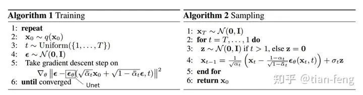
• The above Algorithm 1 represents the training process.

In the second step, data is taken, generally consisting of a category of images, such as cats or dogs, or images of a specific style; it cannot be a random mix of images, or the model won’t learn.

The third step states that each image is randomly assigned a moment of noise (as mentioned earlier).

The fourth step indicates that the noise follows a Gaussian distribution.

The fifth step calculates the loss between the real noise and the predicted noise (the DDPM input does not have a text vector, so it is not written here; you can understand it as having an additional input), updating parameters until the output noise closely matches the real noise, completing the UNet model training.

• Next, we arrive at Algorithm 2, the sampling process.

1. It simply states that Xt follows a Gaussian distribution.

2. Executing T times, we sequentially find Xt-1 to X0, which are T moments.

3. Xt-1 is the formula we derived from reverse diffusion, Xt-1=μ+σZ, where the mean and variance are known, and the only unknown noise Z is predicted by the UNet model.

Sampling Diagram

• To facilitate understanding, I have drawn separate diagrams for text-to-image and image-to-image. Those who use stable diffusion web UI will find them familiar. In text-to-image, we directly initialize a noise and perform sampling.

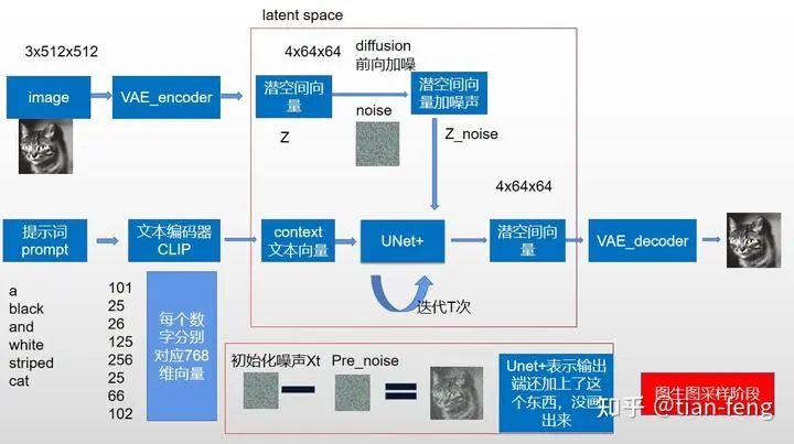
• In image-to-image, noise is added based on your original image, and you control the noise weight. The web UI interface has a redraw amplitude, which corresponds to this.

• The number of iterations corresponds to the sampling steps in the web UI interface.

• The random seed is a noise image we initially obtain randomly, so if you want to replicate the same image, the seed must remain consistent.

Stage Summary

Now let’s take another look at this diagram. Aside from UNet, which I haven’t explained (it will be introduced separately below), isn’t it much simpler? The far left is the pixel space encoder-decoder, and the far right is CLIP converting text into text vectors. The upper middle part is for adding noise, while the lower part is for UNet predicting noise, then continuously sampling to decode and obtain the output image. This is the sampling diagram from the original paper, which doesn’t illustrate the training process.

3. UNet Model

The UNet model is something many of you may have heard of, which involves multi-scale feature fusion, similar to FPN image pyramids, PAN, and many others that share a similar concept. Generally, ResNet is used as the backbone (downsampling) to serve as the encoder, allowing us to obtain multiple scales of feature maps, which are then concatenated during the upsampling process (the feature maps obtained from downsampling). This is a typical UNet.

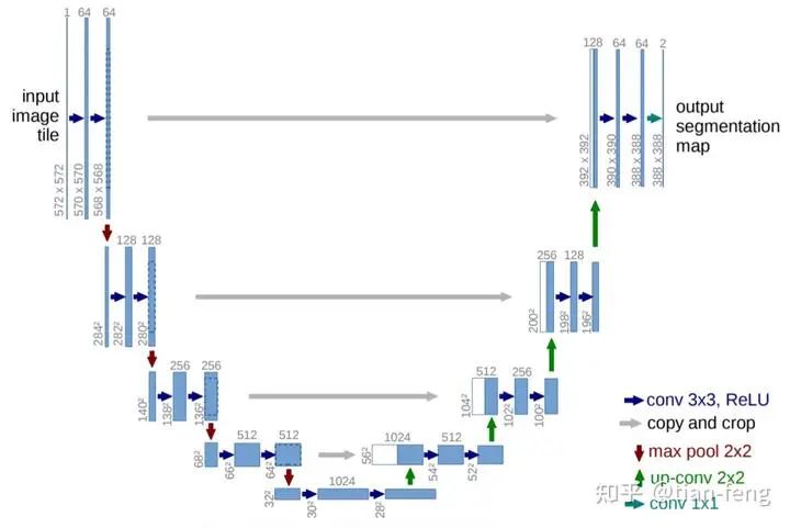
So, what is different about the UNet used in stable diffusion? Here’s a diagram I found, and I admire the patience of this artist, so I borrowed her diagram.

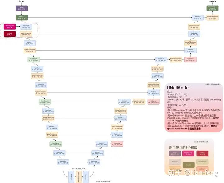
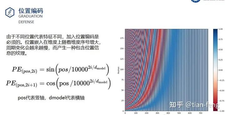
I will explain the ResBlock module and the SpatialTransformer module. The inputs are timestep_embedding, context, and input, which are the three inputs: the time step, text vector, and noisy image. You can understand the time step as positional encoding in transformers, which is used in natural language processing to inform the model of the position of each word in a sentence, as different positions can significantly change the meaning. Here, adding the time step information can be understood as informing the model of the moment when noise is added (of course, this is my interpretation).

Timestep Embedding Uses Sinusoidal Encoding

The ResBlock module takes the time encoding and the convolved image as inputs, outputting their sum. This is its function; I won’t go into the details, as it’s just convolution and fully connected layers, which are quite straightforward.

The SpatialTransformer module takes the text vector and the output from the previous ResBlock as inputs.

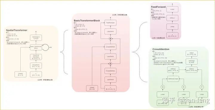
Here, I mainly want to discuss cross-attention. The rest involves some dimensional transformations, convolution operations, and various normalization techniques like Group Norm and Layer Norm.

Using cross-attention, we fuse the features of the latent space with the features of another modal sequence (the text vector) and add them to the reverse process of the diffusion model. Through UNet, we predict the noise that needs to be reduced at each step based on the GT noise and the predicted noise loss function to calculate the gradient.

Looking at the diagram in the lower right corner, we can see that Q represents the features of the latent space, while KV are the text vectors, which are connected through two fully connected layers. The rest is standard transformer operations. After multiplying Q and K, we apply softmax to obtain a score, which is then multiplied by V to transform the dimension and produce the output. You can think of the transformer as a feature extractor that highlights important information (this is just for understanding). That’s roughly how it works, and the subsequent operations are quite similar, ultimately outputting the predicted noise.

Here, you definitely need to be familiar with transformers and know what self-attention and cross-attention are. If you don’t understand, find an article to read; it’s not something that can be simply explained.

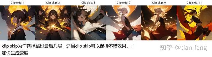
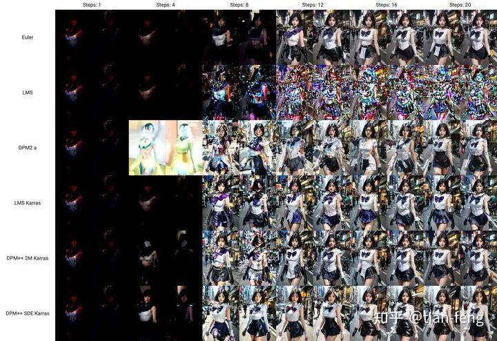
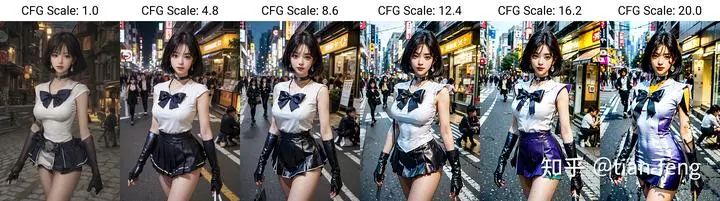
That’s all for now, goodbye! Here are some comparison images from the web UI.

3. Stable Diffusion WebUI Extensions

Parameters for CLIP