This article is excerpted from the latest AI Bible “Deep Learning[1]” published by the People’s Posts and Telecommunications Press. The English version of “Deep Learning[2]” was released by the MIT Press in December 2016 and became popular worldwide upon publication. One of the major features of “Deep Learning[3]” is that it introduces the essence of deep learning algorithms, presenting the logic behind the algorithms without delving into specific code implementations, making it accessible to those who do not write code.
Co-authored by three leading experts in the field of deep learning, Ian Goodfellow, Yoshua Bengio, and Aaron Courville, the AI Bible “Deep Learning[4]” has been at the top of the Amazon AI book charts in the USA for a long time. The Chinese version has filled a gap in the current lack of comprehensive textbooks on deep learning in the country, adding fuel to the hot trend of artificial intelligence.
Readers who wish to purchase this book at the best price can click “Read the Original” to visit our professional bookstore.
Additionally, by this Friday night, the top three comments with the most likes will receive a free copy of this book!
Introduction
As far back as ancient Greece, inventors dreamed of creating machines that could think for themselves. Mythical figures like Pygmalion, Daedalus, and Hephaestus can be seen as legendary inventors, while Galatea, Talos, and Pandora can be viewed as artificial life (Ovid and Martin, 2004; Sparkes, 1996; Tandy, 1997).
When humans first conceived of programmable computers, they were already pondering whether computers could become intelligent (even though it would be over a hundred years before the first computer was built) (Lovelace, 1842). Today, artificial intelligence (AI) has become a field with numerous practical applications and active research topics, and it is flourishing. We expect to automate routine labor through intelligent software, understand speech or images, assist in medical diagnoses, and support fundamental scientific research.
In the early days of AI, problems that were very difficult for human intelligence but relatively simple for computers were solved quickly, such as those that could be described by a series of formal mathematical rules. The real challenge for AI lies in solving tasks that are easy for humans to perform but difficult to formalize, such as recognizing what people say or faces in images. For these problems, we humans can often solve them intuitively and easily.
This book discusses a solution to these more intuitive problems. The solution allows computers to learn from experience and understand the world based on a hierarchical system of concepts, where each concept is defined through relationships with some relatively simple concepts. Allowing computers to gain knowledge from experience avoids the need for humans to formally specify all the knowledge that the computer needs. Hierarchical concepts enable computers to build simpler concepts to learn complex concepts. If we were to draw a diagram illustrating how these concepts build upon one another, we would obtain a “deep” diagram (with many layers). For this reason, we refer to this method as AI deep learning.
Many of AI’s early successes occurred in relatively simple and formalized environments, and did not require computers to possess much knowledge about the world. For example, IBM’s Deep Blue chess system defeated world champion Garry Kasparov in 1997 (Hsu, 2002). Clearly, chess is a very simple domain, as it only contains 64 positions and can only move 32 pieces in strictly limited ways. Designing a successful chess strategy is a tremendous achievement, but describing the pieces and their allowed moves to a computer is not the challenge’s difficulty. Chess can be described by a very short, completely formalized list of rules and can be easily prepared in advance by programmers.
Ironically, abstract and formalized tasks are among the most difficult cognitive tasks for humans, but they are among the easiest for computers. Computers have long been able to defeat the best human chess players, but only recently have they reached human-level performance in object recognition or speech tasks. A person’s daily life requires a vast amount of knowledge about the world. Much of this knowledge is subjective and intuitive, making it difficult to express formally. Computers need to acquire the same knowledge to exhibit intelligence. A key challenge in AI is how to convey this non-formalized knowledge to computers.
Some AI projects strive to hard-code knowledge about the world into formal languages. Computers can use logical reasoning rules to automatically understand statements in these formal languages. This is the well-known knowledge base approach in AI. However, these projects ultimately did not achieve significant success. The most famous project is Cyc (Lenat and Guha, 1989). Cyc includes an inference engine and a database of statements described using the CycL language. These statements are input by human supervisors. This is a cumbersome process. People have managed to design sufficiently complex formal rules to accurately describe the world. For example, Cyc cannot understand a story about a person named Fred shaving in the morning (Linde, 1992). Its inference engine detects inconsistencies in the story: it knows that the composition of a human body does not contain electrical parts, but since Fred is holding an electric razor, it assumes that the entity – “Fred While Shaving” contains electrical components. Therefore, it raises the question – is Fred still a human while shaving?
The difficulties faced by hard-coded knowledge systems indicate that AI systems need to have the ability to acquire knowledge themselves, that is, the ability to extract patterns from raw data. This ability is called machine learning. The introduction of machine learning allows computers to solve problems involving real-world knowledge and to make seemingly subjective decisions. For instance, a simple machine learning algorithm called logistic regression can decide whether to recommend a cesarean section (Mor-Yosef et al., 1990). Similarly, a simple machine learning algorithm called naive Bayes can differentiate between spam emails and legitimate ones.
The performance of these simple machine learning algorithms greatly depends on the representation of the given data. For example, when logistic regression is used to determine whether a patient is suitable for a cesarean section, the AI system does not directly examine the patient. Instead, the doctor needs to inform the system of several relevant pieces of information, such as whether there are uterine scars. Each piece of information representing the patient is called a feature. Logistic regression learns how these features relate to various outcomes. However, it has no influence over how the feature is defined. If the patient’s MRI (magnetic resonance imaging) scan is used as input for logistic regression instead of the doctor’s formal report, it will be unable to make useful predictions. The correlation between a single pixel of the MRI scan and complications during childbirth is negligible.
In computer science and even daily life, the dependence on representation is a common phenomenon. In computer science, if a data set is cleverly structured and intelligently indexed, operations like searching can be processed exponentially faster. People can easily perform arithmetic operations under the representation of Arabic numerals, but it becomes more time-consuming under Roman numerals. Therefore, it is not surprising that the choice of representation has a tremendous impact on the performance of machine learning algorithms. Figure 1.1 presents a simple visual example.
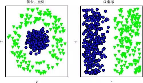
Figure 1.1 Examples of different representations: Suppose we want to draw a line in a scatter plot to separate two classes of data. In the left image, we use Cartesian coordinates to represent the data, and this task is impossible. In the right image, we use polar coordinates to represent the data, and this task can be easily solved with a vertical line (with David Warde-Farley’s collaboration to draw this figure)
Many AI tasks can be solved by first extracting a suitable set of features and then providing those features to a simple machine learning algorithm. For example, for the task of identifying a speaker by voice, a useful feature is an estimate of the size of their vocal tract. This feature provides strong clues for determining whether the speaker is male, female, or a child.
However, for many tasks, it is difficult to know which features to extract. For example, suppose we want to write a program to detect cars in photos. We know that cars have wheels, so we might think to use the presence or absence of wheels as a feature. Unfortunately, we find it challenging to accurately describe what wheels look like based on pixel values. While wheels have simple geometric shapes, their images may vary due to the scene, such as shadows falling on the wheels, shiny metal parts of the wheels illuminated by the sun, the car’s fenders, or foreground objects that partially obscure the wheels.
One approach to solving this problem is to use machine learning to discover the representation itself, rather than just mapping the representation to the output.
We call this approach representation learning. The learned representations often perform better than manually designed representations. Moreover, they require minimal human intervention, allowing AI systems to quickly adapt to new tasks. Representation learning algorithms can discover a good set of features for simple tasks in just a few minutes, while more complex tasks may take hours to months. Manually designing features for a complex task requires a significant amount of human effort, time, and energy, potentially taking decades of research from an entire community of researchers.
A typical example of a representation learning algorithm is the autoencoder. An autoencoder consists of an encoder function and a decoder function. The encoder function transforms the input data into a different representation, while the decoder function transforms this new representation back to its original form. We hope that when the input data passes through the encoder and decoder, as much information as possible is retained, while also expecting that the new representation has various good properties, which is also the training goal of the autoencoder. Different forms of autoencoders can be designed to achieve different properties.
When designing features or algorithms for learning features, our goal is often to isolate the factors of variation that explain the observed data. In this context, the term “factors” refers to different sources of influence; factors are typically not multiplicative combinations. These factors are often unobservable quantities. Instead, they may be unobservable objects in the real world or unobservable forces, but they affect observable quantities. To provide useful simplifications or infer their causes for the observed data, they may also exist in conceptual forms in human thought. They can be seen as concepts or abstractions of the data that help us understand the richness and diversity of these data. When analyzing speech recordings, the factors of variation include the speaker’s age, gender, accent, and the words they are saying. When analyzing images of cars, the factors of variation include the car’s position, color, angle of the sun, and brightness.
In many real-world AI applications, the difficulties mainly arise from multiple factors of variation simultaneously affecting every piece of data we can observe. For example, in an image containing a red car, its individual pixels may be very close to black at night. The shape of the car’s outline depends on the viewing angle. Most applications require us to clarify the factors of variation and ignore those we are not concerned with.
Clearly, extracting such high-level, abstract features from raw data is very difficult. Many factors of variation, such as accents in speech, can only be identified through complex, human-level understanding of the data. This is nearly as challenging as obtaining representations for the original problems, so at first glance, representation learning does not seem to help us.
Deep learning addresses the core problem of representation learning by expressing complex representations through other simpler representations.
Deep learning allows computers to build complex concepts through simpler concepts. Figure 1.2 illustrates how deep learning systems represent the concept of a person in an image by combining simpler concepts (such as angles and contours, which in turn are defined by edges). A typical example of a deep learning model is the feedforward deep network or multilayer perceptron (MLP). A multilayer perceptron is simply a mathematical function that maps a set of input values to output values. This function is composed of many simpler functions. We can think of each application of different mathematical functions as providing a new representation for the input.
The idea of learning the correct representation of data is one perspective for understanding deep learning. Another perspective is that depth encourages the computer to learn a multi-step computer program. Each layer of representation can be thought of as the state of the computer’s memory after executing another set of instructions in parallel. Deeper networks can execute more instructions in sequence. Sequential instructions provide great capability, as later instructions can reference the results of earlier instructions. From this perspective, not all information in the activation function of a layer contains the factors of variation that explain the input. The representation also stores state information to help the program understand the input. Here, the state information is akin to counters or pointers in traditional computer programs. It is unrelated to the specific input content but helps the model organize its processing.
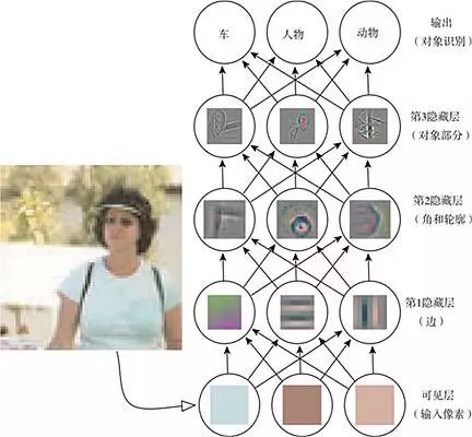
Figure 1.2 A schematic diagram of a deep learning model. Computers struggle to understand the meaning of raw sensory input data, such as images represented as collections of pixel values. Mapping a set of pixels to object identities is a very complex function. If processed directly, learning or evaluating this mapping seems impossible. Deep learning breaks the required complex mapping into a series of nested simple mappings (each described by different layers of the model) to solve this problem. The input is displayed in the visible layer, which is named so because it contains the variables we can observe. Then comes a series of hidden layers that extract increasingly abstract features from the image. Since their values are not provided in the data, these layers are called “hidden layers”; the model must determine which concepts are useful for explaining the relationships in the observed data. The images here visualize the features represented by each hidden unit. Given the pixels, the first layer can easily identify edges by comparing the brightness of adjacent pixels. With the edges described by the first hidden layer, the second hidden layer can easily search for edges that can be recognized as angles and extended contours. Given the image descriptions of angles and contours from the second hidden layer, the third hidden layer can find specific sets of contours and angles to detect entire parts of specific objects. Finally, based on the object parts included in the image descriptions, the model can identify the objects present in the image (this figure is reproduced with permission from Zeiler and Fergus (2014)).
Currently, there are two main ways to measure model depth. One way is based on evaluating the number of sequential instructions the architecture needs to execute. If we represent the model as a flowchart that computes the corresponding output after a given input, we can view the longest path in this flowchart as the model’s depth. Just as two equivalent programs written in different languages will have different lengths, the same function can be drawn as flowcharts of different depths, depending on the functions we can use as a step. Figure 1.3 illustrates how the choice of language gives two different measures of the same architecture.
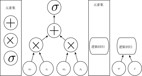
Figure 1.3 A schematic diagram of the computational graph that maps inputs to outputs, where each node performs an operation. The depth is the length of the longest path from input to output, but it depends on the definition of possible computational steps. The computations shown in these graphs are the outputs of a logistic regression model,
σ(wTx), whereσis the logistic sigmoid function. If addition, multiplication, and logistic sigmoid are used as elements of the computer language, then the depth of this model is 3; if logistic regression is viewed as an element itself, then the depth of this model is 1.
Another method used in deep probabilistic models does not view the depth of the computational graph as the model depth, but rather the depth of the graph that describes how concepts relate to one another as the model depth. In this case, the depth of the computational flowchart for each concept representation may be deeper than the graph of the concepts themselves. This is because the system’s understanding of simpler concepts can be further refined after providing information about more complex concepts. For example, when an AI system observes a face image with one eye in shadow, it may initially only see one eye. However, when the presence of a face is detected, the system can infer that the second eye may also be present. In this case, the graph of concepts includes only two layers (the layer about eyes and the layer about faces), but if we refine the estimates for each concept, it would require an additional n computations, making the computational graph contain 2n layers.
Since it is not always clear which is more meaningful – the depth of the computational graph or the depth of the probabilistic model graph – and since different people choose different sets of minimal elements to build their respective graphs, just as there is no single correct value for the length of a computer program, there is also no single correct value for the depth of an architecture. Moreover, there is no consensus on how deep a model must be to be labeled as “deep.” However, it is undeniable that compared to traditional machine learning, deep learning models involve more learned functions or combinations of learned concepts.
In summary, the theme of this book – deep learning is one of the pathways to artificial intelligence. Specifically, it is a type of machine learning, a technology that enables computer systems to improve from experience and data. We firmly believe that machine learning can build AI systems that operate in complex real-world environments and that it is the only practical method. Deep learning is a specific type of machine learning with powerful capabilities and flexibility, representing the vast world as a nested hierarchical system of concepts (where complex concepts are defined by the relationships between simpler concepts, ranging from general abstractions to high-level abstract representations). Figure 1.4 illustrates the relationships between these different AI disciplines. Figure 1.5 presents the high-level principles of how each discipline works.
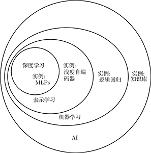
Figure 1.4 A Venn diagram showing that deep learning is both a representation learning and a machine learning method that can be applied to many (but not all) AI methods. Each part of the Venn diagram includes an instance of an AI technology.
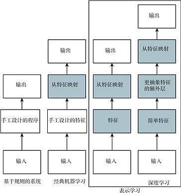
Figure 1.5 A flowchart showing how different parts of AI systems relate to one another across different AI disciplines. The shaded boxes indicate components that can learn from data.
Historical Trends in Deep Learning
Understanding deep learning through its historical context is the simplest way. Here we will only point out a few key trends in deep learning, rather than providing a detailed history:
-
–Deep learning has a long and rich history, but as many different philosophical viewpoints have gradually faded, the corresponding names have also been buried.
-
–As the available training data increases, deep learning becomes more useful.
-
–Over time, the computational hardware and software infrastructure for deep learning have improved, and the scale of deep learning models has grown accordingly.
-
–Over time, deep learning has addressed increasingly complex applications and has continually improved in accuracy.
The Many Names and Fates of Neural Networks
We expect that many readers of this book have heard of deep learning, this exciting new technology, and may be surprised by a book mentioning the “history” of an emerging field. In fact, the history of deep learning can be traced back to the 1940s. Although deep learning seems like a brand-new field, it was relatively obscure in the years leading up to its current popularity, partly because it has been given many different names (most of which are no longer in use) and has only recently become widely known as “deep learning.” This field has changed names many times, reflecting the influence of different researchers and perspectives.
Telling the full history of deep learning is beyond the scope of this book. However, some basic background is useful for understanding deep learning. It is generally believed that deep learning has gone through three waves of development: from the 1940s to the 1960s, the early forms of deep learning appeared in cybernetics; from the 1980s to the 1990s, deep learning manifested as connectionism; and it was not until 2006 that it truly revived under the name of deep learning. Figure 1.7 provides a quantitative visualization.
Some of the earliest learning algorithms we know today aimed to simulate biological learning computational models, i.e., models of how the brain learns or why it can learn. As a result, deep learning faded under the name of artificial neural networks (ANN). At that time, deep learning models were seen as systems inspired by biological brains (whether human brains or those of other animals). Although some machine learning neural networks were sometimes used to understand brain functions (Hinton and Shallice, 1991), they were generally not designed to be true models of biological functions. The neural perspective of deep learning was inspired by two main ideas: one idea is that the brain serves as an example proving that intelligent behavior is possible, thus conceptually, the direct way to establish intelligence is to reverse-engineer the computational principles behind the brain and replicate its functions; another view is that understanding the principles behind the brain and human intelligence is also very interesting, so machine learning models, in addition to their ability to solve engineering applications, would also be useful if they could lead to further insights into these fundamental scientific questions.
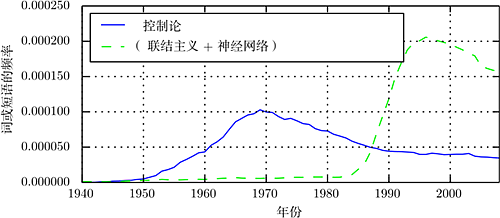
Figure 1.7 The historical waves of research on artificial neural networks measured by the frequency of the phrases “cybernetics,” “connectionism,” or “neural networks” in Google Books (the figure shows the first two waves, with the third wave appearing only recently). The first wave began with cybernetics from the 1940s to the 1960s, coinciding with the development of biological learning theories (McCulloch and Pitts, 1943; Hebb, 1949) and the implementation of the first models (such as the perceptron (Rosenblatt, 1958)), which enabled the training of individual neurons. The second wave began with the connectionist approaches from 1980 to 1995, which could train neural networks with one or two hidden layers using backpropagation (Rumelhart et al., 1986a). The current third wave, deep learning, began around 2006 (Hinton et al., 2006a; Bengio et al., 2007a; Ranzato et al., 2007a) and emerged in book form in 2016. Additionally, the first two waves similarly appeared in books much later than the corresponding scientific activities.
The modern term “deep learning” transcends the neural science perspective of current machine learning models. It appeals to the more general principle of learning multi-layered combinations, which can also be applied to machine learning frameworks that are not inspired by neuroscience.
The earliest predecessors of modern deep learning emerged from simple linear models from a neuroscience perspective. These models were designed to use a set of n inputs x1, ··· , xn and associate them with an output y. These models aimed to learn a set of weights w1, ··· , wn and calculate their output f(x,w) = x1w1 + ··· + xnwn. As shown in Figure 1.7, the first wave of neural network research is called cybernetics.
The McCulloch-Pitts neuron (McCulloch and Pitts, 1943) was an early model of brain function. This linear model identified two different categories of inputs by examining the sign of the function f(x,w). Clearly, the model’s weights need to be set correctly for the model’s output to correspond to the expected category. These weights can be set by an operator. In the 1950s, the perceptron (Rosenblatt, 1956, 1958) became the first model capable of learning weights based on input samples from each category. Around the same period, the adaptive linear element (ADALINE) simply returned the value of the function f(x) itself to predict a real number (Widrow and Hoff, 1960), and it could also learn to predict these numbers from data.
These simple learning algorithms significantly influenced the modern landscape of machine learning. The training algorithm used to adjust the weights of ADALINE is a special case of what is called stochastic gradient descent. The slightly improved stochastic gradient descent algorithm remains the primary training algorithm for deep learning today.
The models based on the function f(x,w) used in perceptrons and ADALINE are called linear models. While these models are trained in ways different from the original models in many cases, they remain the most widely used machine learning models today.
Linear models have many limitations. The most famous is that they cannot learn the XOR (exclusive OR) function, i.e., f([0,1],w) = 1 and f([1,0],w) = 1, but f([1,1],w) = 0 and f([0,0],w) = 0. Observing this flaw in linear models led critics to develop a general aversion to biologically inspired learning (Minsky and Papert, 1969). This resulted in the first major decline of the neural network craze.
Now, neuroscience is viewed as an important source of inspiration for deep learning research, but it is no longer the field’s primary guide.
Today, the role of neuroscience in deep learning research has been diminished, primarily because we do not have sufficient information about the brain to guide its use. To gain a profound understanding of the algorithms actually used by the brain, we need to be able to simultaneously monitor the activities of (at least) thousands of interconnected neurons. We are not able to do this, so we do not even fully understand the simplest and most well-studied parts of the brain (Olshausen and Field, 2005).
Neuroscience has provided us with reasons to believe that a single deep learning algorithm can solve many different tasks. Neuroscientists have found that if the brains of ferrets are rewired to transmit visual signals to the auditory region, they can learn to “see” using the auditory processing region of the brain (Von Melchner et al., 2000). This suggests that the brains of most mammals can use a single algorithm to solve most of the different tasks their brains can handle. Before this assumption, machine learning research was relatively fragmented, with researchers studying natural language processing, computer vision, motion planning, and speech recognition in different communities. Today, while these application communities remain independent, it is common for deep learning research groups to simultaneously study many or even all of these application areas.
We can glean some rough guidelines from neuroscience. The basic idea that intelligence emerges from the interactions between computational units is inspired by the brain. The new cognitive model (Fukushima, 1980) was inspired by the structure of the mammalian visual system, introducing a powerful model architecture for processing images, which later became the basis for modern convolutional networks (LeCun et al., 1998c) (see Section 9.10). Most neural networks today are based on a neural unit model known as the rectified linear unit. The original cognitive model (Fukushima, 1975) was inspired by our knowledge of brain function, introducing a more complex version. The simplified modern version has formed by absorbing ideas from different perspectives, with Nair and Hinton (2010b) and Glorot et al. (2011a) citing neuroscience as an influence, while Jarrett et al. (2009a) cited more engineering-oriented influences. Although neuroscience is an important source of inspiration, it should not be viewed as rigid guidance. We know that real neurons compute functions very different from modern rectified linear units, but systems that are closer to real neural networks have not led to improvements in machine learning performance. Additionally, while neuroscience has successfully inspired some neural network architectures, we do not have enough understanding of biological learning for neuroscience to provide much guidance for the learning algorithms used to train these architectures.
The media often emphasizes the similarities between deep learning and the brain. Indeed, deep learning researchers are more likely than researchers in other machine learning fields (such as kernel methods or Bayesian statistics) to cite the brain as an influence, but one should not assume that deep learning is attempting to simulate the brain. Modern deep learning draws inspiration from many fields, particularly the fundamentals of applied mathematics, such as linear algebra, probability theory, information theory, and numerical optimization. While some deep learning researchers cite neuroscience as an important source of inspiration, other scholars may be entirely indifferent to neuroscience.
It is noteworthy that attempts to understand how the brain works at the algorithmic level do exist and are progressing well. This effort is mainly known as “computational neuroscience” and is an independent field from deep learning. Researchers often move back and forth between the two fields. The deep learning field primarily focuses on building computer systems that can successfully solve tasks requiring intelligence, while the computational neuroscience field mainly focuses on constructing accurate models of how the brain actually works.
In the 1980s, the second wave of neural network research largely accompanied a trend known as connectionism or parallel distributed processing (Rumelhart et al., 1986d; McClelland et al., 1995). Connectionism emerged in the context of cognitive science. Cognitive science is an interdisciplinary approach to understanding thought, integrating multiple different levels of analysis. In the early 1980s, most cognitive scientists studied symbolic reasoning models. Although this was popular, symbolic models struggled to explain how the brain actually uses neurons to achieve reasoning functions.
Connectionists began to study cognitive models based on the actual implementation in the nervous system (Touretzky and Minton, 1985), many of which revived ideas that can be traced back to psychologist Donald Hebb’s work in the 1940s (Hebb, 1949).
The central idea of connectionism is that intelligence can emerge when large numbers of simple computational units are connected together. This insight also applies to neurons in biological nervous systems, as they serve a similar role to hidden units in computational models.
Several key concepts formed during the connectionist wave of the 1980s remain very important in today’s deep learning.
One of these concepts is distributed representation (Hinton et al., 1986). The idea is that each input to the system should be represented by multiple features, and each feature should be involved in the representation of multiple possible inputs. For example, suppose we have a visual system that can recognize red, green, or blue cars, trucks, and birds. One way to represent these inputs is to activate nine different neurons or hidden units for each of the nine possible combinations: red truck, red car, red bird, green truck, etc. This requires nine different neurons, and each neuron must independently learn the concepts of color and object identity. One way to improve this situation is to use distributed representation, which describes color with three neurons and object identity with three neurons. This only requires six neurons instead of nine, and the neurons representing red can learn the color from images of cars, trucks, and birds, rather than just from images of one specific category. The concept of distributed representation is central to this book, and we will describe it in more detail in Chapter 15.
Another important achievement of the connectionist wave is the successful use of backpropagation in training deep neural networks with internal representations and the popularization of the backpropagation algorithm (Rumelhart et al., 1986c; LeCun, 1987). Although this algorithm fell into obscurity and was no longer popular, as of the time of writing this book, it remains the dominant method for training deep models.
In the 1990s, researchers made significant advances in using neural networks for sequence modeling. Hochreiter (1991b) and Bengio et al. (1994b) identified some fundamental mathematical challenges in modeling long sequences, which will be described in Section 10.7. Hochreiter and Schmidhuber (1997) introduced long short-term memory (LSTM) networks to address these challenges. Today, LSTMs are widely used in many sequence modeling tasks, including many natural language processing tasks by Google.
The second wave of neural network research continued until the mid-1990s. Startups based on neural networks and other AI technologies sought investment, with ambitious but unrealistic approaches. When AI research failed to meet these unreasonable expectations, investors became disappointed. Meanwhile, other fields of machine learning made progress. For example, kernel methods (Boser et al., 1992; Cortes and Vapnik, 1995; Schölkopf et al., 1999) and graphical models (Jordan, 1998) achieved good results on many important tasks. These two factors led to the second decline of the neural network craze, which lasted until 2007.
During this period, neural networks continued to achieve impressive performance on certain tasks (LeCun et al., 1998c; Bengio et al., 2001a). The Canadian Institute for Advanced Research (CIFAR) helped sustain neural network research through its Neural Computation and Adaptive Perception (NCAP) research program. This program brought together machine learning research groups led by Geoffrey Hinton, Yoshua Bengio, and Yann LeCun at the University of Toronto, the University of Montreal, and New York University, respectively. This multidisciplinary CIFAR NCAP research program also included neuroscientists, human and computer vision experts.
At that time, it was widely believed that deep networks were difficult to train. Now we know that the algorithms existing since the 1980s work very well, but it was not until around 2006 that this became apparent. This may simply be due to the computational costs being too high, making it difficult to conduct sufficient experiments with the hardware available at that time.
The third wave of neural network research began with breakthroughs in 2006. Geoffrey Hinton demonstrated that a neural network called the “deep belief network” could be effectively trained using a strategy called “greedy layer-wise pre-training” (Hinton et al., 2006a), which we will describe in more detail in Section 15.1. Other CIFAR-affiliated research groups quickly demonstrated that the same strategy could be used to train many other types of deep networks (Bengio and LeCun, 2007a; Ranzato et al., 2007b) and systematically help improve generalization on test samples. This wave of neural network research popularized the term “deep learning,” emphasizing that researchers now had the ability to train previously untrainable deeper neural networks and focusing on the theoretical importance of depth (Bengio and LeCun, 2007b; Delalleau and Bengio, 2011; Pascanu et al., 2014a; Montufar et al., 2014). By this time, deep neural networks had surpassed competing AI systems based on other machine learning techniques and hand-designed functions. As of the time of writing this book, the third wave of neural network development is still ongoing, although the focus of deep learning research has changed significantly during this period. The third wave has begun to look at new unsupervised learning techniques and the generalization capabilities of deep models on small datasets, but currently, more interest remains in the capabilities of traditional supervised learning algorithms and deep models to fully utilize large labeled datasets.
Increasing Amounts of Data
One might ask, since the first experiments with artificial neural networks were conducted in the 1950s, why has deep learning only recently been considered a key technology? Since the 1990s, deep learning has been successfully applied in commercial applications, but it was often seen as an art that only experts could use rather than a technology, a view that persisted until recently. Indeed, obtaining good performance from a deep learning algorithm requires some skill. Fortunately, as the amount of training data increases, the required skills are decreasing. Current learning algorithms that achieve human-level performance on complex tasks are almost identical to those that struggled to solve toy problems in the 1980s, even though the models trained with these algorithms have undergone transformations, simplifying the training of extremely deep architectures. The most important new development is that we now have the resources required for successfully training these algorithms. Figure 1.8 illustrates how the size of benchmark datasets has significantly increased over time.
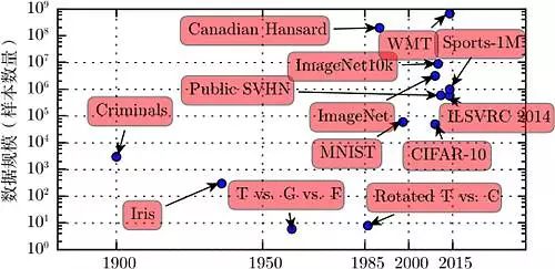
Figure 1.8 Increasing amounts of data. In the early 20th century, statisticians used hundreds or thousands of manually created metrics to study datasets (Garson, 1900; Gosset, 1908; Anderson, 1935; Fisher, 1936). From the 1950s to the 1980s, pioneers of biologically inspired machine learning typically used small synthetic datasets, such as low-resolution letter bitmaps, designed to demonstrate that neural networks could learn specific functions at low computational costs (Widrow and Hoff, 1960; Rumelhart et al., 1986b). From the 1980s to the 1990s, machine learning became more statistical and began utilizing larger datasets containing thousands of samples, such as the MNIST dataset of handwritten scanned digits (as shown in Figure 1.9) (LeCun et al., 1998c). In the first decade of the 21st century, similarly sized but more complex datasets continued to emerge, such as the CIFAR-10 dataset (Krizhevsky and Hinton, 2009). At the end of this decade and in the following five years, significantly larger datasets (containing tens of thousands to millions of samples) completely changed what deep learning could achieve. These datasets include the public Street View House Numbers dataset (Netzer et al., 2011), various versions of the ImageNet dataset (Deng et al., 2009, 2010a; Russakovsky et al., 2014a), and the Sports-1M dataset (Karpathy et al., 2014). At the top of the figure, we see that datasets for translating sentences are often larger than other datasets, such as the IBM dataset based on the Canadian Hansard (Brown et al., 1990) and the WMT 2014 English-French dataset (Schwenk, 2014).
This trend is driven by the increasing digitization of society. As our activities increasingly take place on computers, what we do is also increasingly recorded. As computers become more interconnected, these records become easier to manage centrally and are easier to organize into datasets suitable for machine learning applications. Because the main burden of statistical estimation (observing a small amount of data to generalize on new data) has been alleviated, the “big data” era has made machine learning easier. As of 2016, a rough rule of thumb is that supervised deep learning algorithms typically achieve acceptable performance when given about 5000 labeled samples per class, and when at least 10 million labeled samples are used for training, they reach or exceed human performance. Additionally, achieving success on smaller datasets is an important research area, for which we should particularly focus on how to make full use of large amounts of unlabeled samples through unsupervised or semi-supervised learning.
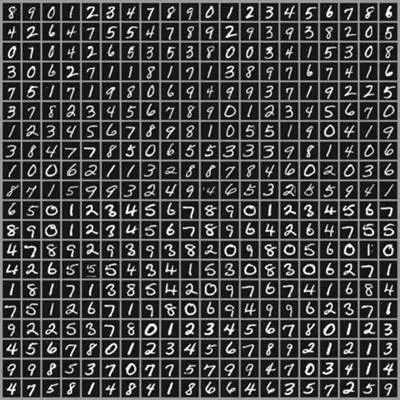
Figure 1.9 Examples of inputs from the MNIST dataset. “NIST” stands for the National Institute of Standards and Technology, which was the original agency that collected this data. “M” stands for “Modified“, indicating that the data has been preprocessed to make it easier to use with machine learning algorithms. The MNIST dataset consists of scanned images of handwritten digits and associated labels (describing which digit from 0 to 9 is contained in each image). This simple classification problem is one of the simplest and most widely used tests in deep learning research. Although modern techniques easily solve this problem, it remains popular. Geoffrey Hinton has described it as the “fruit fly of machine learning,” meaning that machine learning researchers can study their algorithms under controlled laboratory conditions, just as biologists often study fruit flies.
Increasing Model Sizes
Another important reason why neural networks have become very successful today, compared to the relatively small successes of neural networks in the 1980s, is that we now have the computational resources to run larger models. One of the main insights of connectionism is that intelligence emerges when many neurons in animals work together. Individual neurons or small sets of neurons are not particularly useful.
Biological neurons are not particularly densely connected. As shown in Figure 1.10, for decades, the number of connections per neuron in our machine learning models has been on the same order of magnitude as that in the mammalian brain.
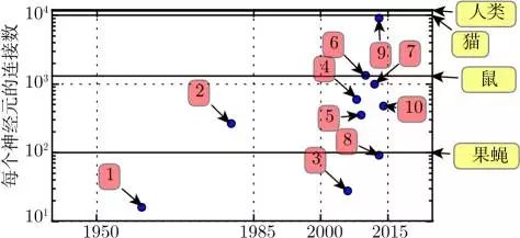
Figure 1.10 Increasing number of connections per neuron. Initially, the number of connections between neurons in artificial neural networks was limited by hardware capabilities. Now, the number of connections between neurons is mostly a design consideration. Some artificial neural networks have as many connections per neuron as a cat, and for others, it is common for each neuron to have as many connections as smaller mammals (like mice). Even the number of connections per neuron in the human brain is not excessively high. The scale of biological neural networks is from Wikipedia (2015).
1. Adaptive Linear Element (Widrow and Hoff, 1960); 2. Neural Cognitive Model (Fukushima, 1980); 3. GPU-accelerated Convolutional Networks (Chellapilla et al., 2006); 4. Deep Boltzmann Machines (Salakhutdinov and Hinton, 2009a); 5. Unsupervised Convolutional Networks (Jarrett et al., 2009b); 6. GPU-accelerated Multilayer Perceptrons (Ciresan et al., 2010); 7. Distributed Autoencoders (Le et al., 2012); 8. Multi-GPU Convolutional Networks (Krizhevsky et al., 2012a); 9. COTS HPC Unsupervised Convolutional Networks (Coates et al., 2013); 10. GoogLeNet (Szegedy et al., 2014a)
As shown in Figure 1.11, until recently, neural networks were remarkably small in terms of total neuron numbers. Since the introduction of hidden units, the scale of artificial neural networks has roughly doubled every 2.4 years. This growth is driven by larger memory, faster computers, and larger available datasets. Larger networks can achieve higher accuracy on more complex tasks. This trend appears to continue for decades. Unless we are able to rapidly scale new technologies, it may take until the 2050s for artificial neural networks to have a comparable number of neurons to the human brain. The functions represented by biological neurons may be more complex than those currently represented by artificial neurons, so biological neural networks may be even larger than depicted in the figure.
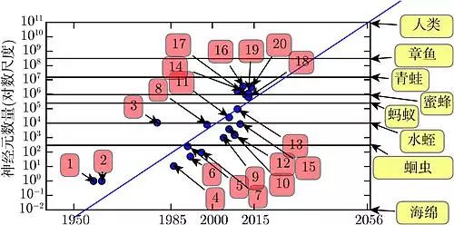
Figure 1.11 Increasing scale of neural networks. Since the introduction of hidden units, the scale of artificial neural networks has roughly doubled every 2.4 years. The scale of biological neural networks is from Wikipedia (2015).
1. Perceptron (Rosenblatt, 1958, 1962); 2. Adaptive Linear Element (Widrow and Hoff, 1960); 3. Neural Cognitive Model (Fukushima, 1980); 4. Early Backpropagation Networks (Rumelhart et al., 1986b); 5. Recurrent Neural Networks for Speech Recognition (Robinson and Fallside, 1991); 6. Multilayer Perceptrons for Speech Recognition (Bengio et al., 1991); 7. Uniform Field Sigmoid Belief Networks (Saul et al., 1996); 8. LeNet5 (LeCun et al., 1998c); 9. Echo State Networks (Jaeger and Haas, 2004); 10. Deep Belief Networks (Hinton et al., 2006a); 11. GPU-accelerated Convolutional Networks (Chellapilla et al., 2006); 12. Deep Boltzmann Machines (Salakhutdinov and Hinton, 2009a); 13. GPU-accelerated Deep Belief Networks (Raina et al., 2009a); 14. Unsupervised Convolutional Networks (Jarrett et al., 2009b); 15. GPU-accelerated Multilayer Perceptrons (Ciresan et al., 2010); 16. OMP-1 Networks (Coates and Ng, 2011); 17. Distributed Autoencoders (Le et al., 2012); 18. Multi-GPU Convolutional Networks (Krizhevsky et al., 2012a); 19. COTS HPC Unsupervised Convolutional Networks (Coates et al., 2013); 20. GoogLeNet (Szegedy et al., 2014a)
Now, it is not surprising that neural networks with fewer neurons than a leech cannot solve complex artificial intelligence problems. Even current networks, from a computational system perspective, may be quite large, but in reality, they are smaller than the nervous systems of relatively primitive vertebrates (such as frogs).
Due to faster CPUs, the advent of general-purpose GPUs, faster network connections, and better distributed computing software infrastructure, the increasing model scale is one of the most important trends in the history of deep learning. This trend is widely expected to continue well into the future.
Increasing Accuracy, Complexity, and Impact on the Real World
Since the 1980s, the ability of deep learning to provide precise recognition and prediction has been steadily increasing. Moreover, deep learning has successfully been applied to an increasingly wide range of practical problems.
The earliest deep models were used to recognize single objects in cropped, compact, and very small images (Rumelhart et al., 1986d). Since then, the sizes of images that neural networks can handle have gradually increased. Modern object recognition networks can process rich, high-resolution photographs without needing to crop around the objects being recognized (Krizhevsky et al., 2012b). Similarly, the earliest networks could only recognize two objects (or in some cases, the presence or absence of a single class of objects), while these modern networks can typically recognize at least 1000 different classes of objects. The biggest competition in object recognition is the annual ImageNet Large Scale Visual Recognition Challenge (ILSVRC). An exciting moment in the rapid rise of deep learning is when convolutional networks first dramatically won this challenge, reducing the top-5 error rate from 26.1% to 15.3% (Krizhevsky et al., 2012b), meaning that the convolutional network generated a sequential list of possible categories for each image, with the correct class label appearing in the top 5 for all test samples except for 15.3%. Since then, deep convolutional networks have consistently won these competitions, and as of the time of writing this book, the latest results have reduced the top-5 error rate in this competition to 3.6%, as shown in Figure 1.12.
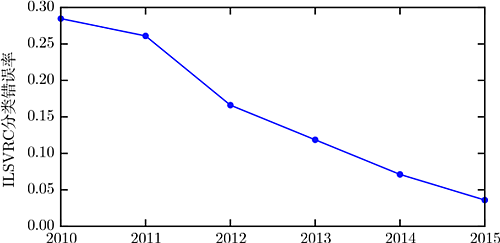
Figure 1.12 Decreasing error rates. As deep networks reached the scale necessary to compete in the ImageNet Large Scale Visual Recognition Challenge, they have won year after year, producing increasingly lower error rates. Data sources are Russakovsky et al. (2014b) and He et al. (2015).
Deep learning has also had a significant impact on speech recognition. After improvements in the 1990s, speech recognition stagnated until around 2000. The introduction of deep learning (Dahl et al., 2010; Deng et al., 2010b; Seide et al., 2011; Hinton et al., 2012a) caused a sharp decline in speech recognition error rates, with some error rates even halving. We will discuss this history in more detail in Section 12.3.
Deep networks have also achieved remarkable successes in pedestrian detection and image segmentation (Sermanet et al., 2013; Farabet et al., 2013; Couprie et al., 2013), and they have outperformed humans in traffic sign classification (Ciresan et al., 2012).
As the scale and accuracy of deep networks have increased, the tasks they can solve have also become increasingly complex. Goodfellow et al. (2014d) demonstrated that neural networks could learn to output entire sequences of characters describing an image, rather than just recognizing individual objects. Previously, it was generally believed that such learning required labeling individual elements in the sequence (Gulcehre and Bengio, 2013). Recurrent neural networks, such as the previously mentioned LSTM sequence model, are now used to model relationships between sequences and other sequences, rather than just relationships between fixed inputs. This sequence-to-sequence learning seems to lead to another disruptive development in applications, namely machine translation (Sutskever et al., 2014; Bahdanau et al., 2015).
This trend of increasing complexity has led to logical conclusions, such as the introduction of the neural Turing machine (Graves et al., 2014), which can learn to read from and write arbitrary content to storage units. Such neural networks can learn simple programs from samples of desired behavior. For example, they can learn to sort a series of numbers from scrambled and sorted samples. This self-programming technique is still in its infancy, but in principle, it could be applied to nearly all tasks in the future.
Another major achievement of deep learning is its expansion into the field of reinforcement learning. In reinforcement learning, an autonomous intelligent agent must learn to perform tasks through trial and error without human operator guidance. DeepMind has shown that deep learning-based reinforcement learning systems can learn to play Atari video games and compete with humans in various tasks (Mnih et al., 2015). Deep learning has also significantly improved the performance of robotic reinforcement learning (Finn et al., 2015).
Many deep learning applications are highly profitable. Deep learning is now used by many top technology companies, including Google, Microsoft, Facebook, IBM, Baidu, Apple, Adobe, Netflix, NVIDIA, and NEC.
Advances in deep learning have also heavily relied on progress in software infrastructure. Software libraries such as Theano (Bergstra et al., 2010a; Bastien et al., 2012a), PyLearn2 (Goodfellow et al., 2013e), Torch (Collobert et al., 2011b), DistBelief (Dean et al., 2012), Caffe (Jia, 2013), MXNet (Chen et al., 2015), and TensorFlow (Abadi et al., 2015) have supported significant research projects or commercial products.
Deep learning has also contributed to other sciences. Modern convolutional networks used for object recognition have provided neuroscientists with models for studying visual processing (DiCarlo, 2013). Deep learning has also provided very useful tools for processing massive data and making effective predictions in scientific fields. It has been successfully used to predict how molecules interact, thereby helping pharmaceutical companies design new drugs (Dahl et al., 2014), search for subatomic particles (Baldi et al., 2014), and automatically parse microscope images used to construct three-dimensional maps of the human brain (Knowles-Barley et al., 2014). We look forward to deep learning appearing in more and more scientific fields in the future.
In summary, deep learning is a method of machine learning. Over the past few decades, it has drawn heavily on our knowledge of the brain, statistics, and applied mathematics. In recent years, thanks to more powerful computers, larger datasets, and techniques capable of training deeper networks, the popularity and practicality of deep learning have seen tremendous growth. In the coming years, deep learning is full of challenges and opportunities for further improvement and application to new fields.
About the Book “Deep Learning”
The Chinese version of “Deep Learning” took three years from copyright introduction to official publication, filling the current gap of comprehensive textbooks on deep learning in the country. The book introduces basic mathematical knowledge, machine learning experience, and the current theories and developments in deep learning from shallow to deep, helping enthusiasts and professionals in artificial intelligence technology to gain a comprehensive understanding of deep learning under the guidance of three expert scholars.
This book is useful for various readers, but it is primarily written for two types of audiences. One type of audience is university students (undergraduate or graduate) learning machine learning, including those who have already started their careers as deep learning and AI researchers. The other type of audience is software engineers without a background in machine learning or statistics who wish to quickly grasp knowledge in this area and use deep learning in their products or platforms. It has been proven that deep learning is useful in many software fields, including computer vision, speech and audio processing, natural language processing, robotics, bioinformatics and chemistry, video games, search engines, online advertising, and finance.
To better serve various readers, we have organized this book into three parts. Part 1 introduces the basic mathematical tools and concepts of machine learning. Part 2 covers the most mature deep learning algorithms, which have essentially been solved. Part 3 discusses certain promising ideas that are widely considered to be the future research focus of deep learning.
Readers can skip sections that are not of interest or unrelated to their background. Readers familiar with linear algebra, probability, and basic machine learning concepts can skip Part 1. If readers only want to implement a working system, they do not need to read beyond Part 2. To help readers choose chapters, the following diagram presents a flowchart of the high-level organization structure of this book.
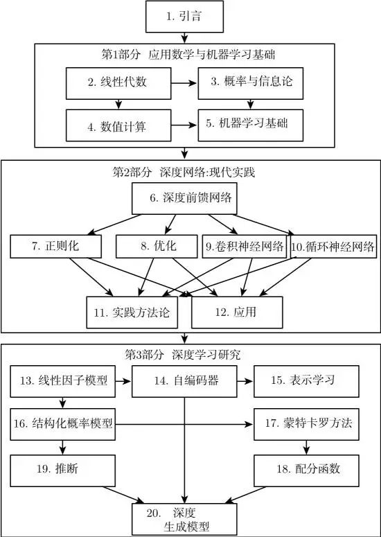
The flowchart of the high-level organization structure of this book. The arrows from one chapter to another indicate that the previous chapter is essential for understanding the subsequent chapter.
We assume that all readers have a background in computer science. We also assume that readers are familiar with programming and have a basic understanding of performance issues in computing, complexity theory, introductory calculus, and some graph theory terminology.
The accompanying website for the English version of “Deep Learning” is www.deeplearningbook.org[5]. The website provides various supplementary materials, including exercises, lecture slides, errata, and other resources that should be useful to readers and instructors.
Readers of the Chinese version of “Deep Learning” can visit the asynchronous community website of the People’s Posts and Telecommunications Press www.epubit.com.cn[6] for more book information.
Readers who wish to purchase this book at the best price can click “Read the Original” to visit our professional bookstore.
Additionally, by this Friday night, the top three comments with the most likes will receive a free copy of this book!