This article was first published on WeChat public account: “The Beauty of Algorithms and Programming”, welcome to follow for more timely updates on this series of articles.
Problem Description
Here is an example of recognizing the mnist handwritten dataset. This dataset is a classic dataset in machine learning, consisting of 60k training samples and 10k testing samples, where each sample is a 28*28 pixel grayscale handwritten digit image. These high-dimensional images cannot be implemented using a linear model; therefore, a nonlinear model is required. Below, we will complete this example through method introduction and code examples.
Method Introduction:
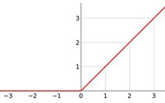
Due to the inability of the linear model to meet the recognition needs of the dataset, we need to introduce an activation function (Relu function) to incorporate non-linear factors. If this still does not meet the needs, we can increase complexity by chaining nonlinear layers to achieve an output like this: out=relu{relu{relu[X@W1+b1]@W2+b2}@W3+b3}. As shown in Figure 1, is the model of the Relu function.
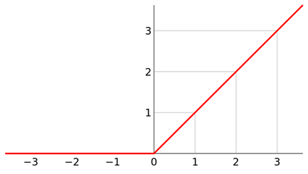
Figure 1 Relu function model
Solution
1.Import tensorflow as tf, get the dataset
|
import tensorflow as tf from tensorflow import keras from tensorflow.keras import datasets (x,y),_ = datasets.mnist.load_data() |
2.Create tensor
Convert numpy to tensor, and adjust the x values from 0~255 to 0~1 by dividing by 255.
|
x = tf.convert_to_tensor(x,dtype=tf.float32) / 255. y = tf.convert_to_tensor(y,dtype=tf.int32) print(tf.reduce_min(x),tf.reduce_max(x)) #checkx min and max values print(tf.reduce_min(y),tf.reduce_max(y)) #checky min and max values |
3.Create dataset
Get 128 samples at a time in batches, making the data iterable by continuously calling the next method.
|
train_db = tf.data.Dataset.from_tensor_slices((x,y)).batch(128) train_iter = iter(train_db) #iterator for continuous callsnext sample = next(train_iter) print(‘batch:’,sample[0].shape,sample[1].shape) |
4.Define parameters and learning rate
Randomly generate parameters with dimensions of [784,256] using the tf.random.truncated_normal() method, where stddev is the standard deviation of the normal distribution; lr is the learning rate.
|
w1 = tf.Variable(tf.random.truncated_normal([784,256],stddev=0.1)) #stddev sets the standard deviation b1 = tf.Variable(tf.zeros([256])) w2 = tf.Variable(tf.random.truncated_normal([256,128],stddev=0.1)) b2 = tf.Variable(tf.zeros([128])) w3 = tf.Variable(tf.random.truncated_normal([128,10],stddev=0.1)) b3 = tf.Variable(tf.zeros([10])) lr=1e-3 |
5.Loop through the dataset
Put the training process inside with tf.GradientTape() as tape, then use tape.gradient() to automatically compute gradients, looping through the dataset in batches using for step, and repeat the entire dataset for ten iterations.
|
for epoch in range(10): # iterate db for 10 # loop through the dataset in batches for step,(x,y) in enumerate(train_db): # for every batch # x:[128,28,28] # y:[128] # [b,28,28] => [b,28*28] # convert x to[batch,784] x = tf.reshape(x,[-1,28*28])
# tensor provides automatic differentiation # put the training process insidewith tf.GradientTape() as tape, then use tape.gradient() to automatically compute gradients with tf.GradientTape() as tape: # tf.Variable # x:[b,28*28] # h1 = x @ w1 + b1 # [b,784] @ [784,256] + [256] => [b,256] + [256] => [b,256] + [256] h1 = x @ w1 + tf.broadcast_to(b1,[x.shape[0],256]) # Non-linear activation h1 = tf.nn.relu(h1) #[b,256] => [b,128] h2 = h1 @ w2 + b2 h2 = tf.nn.relu(h2) # [b,128] => [b,10] out = h2 @ w3 + b3
# compute loss # out:[b,10] # y:[b] => [b,10] y_onehot = tf.one_hot(y,depth=10)
# mse = mean(sum(y-out)**2) # [b,10] loss = tf.square(y_onehot – out) # mean:scalar loss = tf.reduce_mean(loss) |
6.Pass the loss function
Pass the loss function and parameters, and update the data using the gradient descent method.
|
grads = tape.gradient(loss,[w1,b1,w2,b2,w3,b3]) # w1 = w1 – lr * w1_grad w1.assign_sub(lr * grads[0]) b1.assign_sub(lr * grads[1]) w2.assign_sub(lr * grads[2]) b2.assign_sub(lr * grads[3]) w3.assign_sub(lr * grads[4]) b3.assign_sub(lr * grads[5]) |
7.Input loss value
|
if step % 100 == 0: print(epoch,step,’loss:’,float(loss)) |
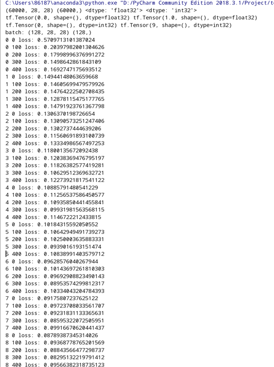
Output Result:
Editor: Wang Nanlan
Source: Deep Learning and Cultural Tourism Application Laboratory (DLETA)