Summary of Hessian Matrix Applications in XGBoost Algorithm

Introduction

The most common application of the Hessian matrix is in the Newton optimization method, which mainly seeks the extremum points of a function where the first derivative is zero. This article provides a straightforward summary of the two applications of the Hessian matrix in the XGBoost algorithm, namely the minimum child weight algorithm and the weight quantile algorithm.

Table of Contents

1. Definition of Hessian Matrix

2. Minimum Child Weight Algorithm

3. Weight Quantile Algorithm

4. Conclusion

1. Definition of Hessian Matrix

The Hessian matrix (Hessian matrix or Hessian) is a square matrix of second-order partial derivatives of a real-valued function with respect to its vector variables, defined as follows:

The independent variable is a vector:

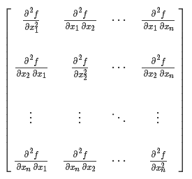
Thus, the Hessian matrix H(f) is defined as:

2. Minimum Child Weight Algorithm

The official documentation defines the parameter minimum child weight (min_child_weight) in the XGBoost algorithm as:

minimum sum of instance weight (hessian) needed in a child. If the tree partition step results in a leaf node with the sum of instance weight less than min_child_weight, then the building process will give up further partitioning. In linear regression mode, this simply corresponds to minimum number of instances needed to be in each node. The larger, the more conservative the algorithm will be.

Translation: min_child_weight is defined as the minimum sum of instance weights (hessian) in a leaf node. If the sum of instance weights in a leaf node is less than min_child_weight, the partitioning process will stop. In the linear regression model, the minimum number of instances reflects the minimum sum of instance weights in a leaf node. The larger the min_child_weight, the more conservative the model becomes, thus reducing model complexity and avoiding overfitting.

Next, we discuss the meaning of using the Hessian to represent node instance weights in tree models and linear models.

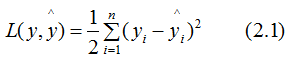
Do you remember the definition of the Hessian matrix? The Hessian is the second derivative of the function value with respect to the variables. In the XGBoost algorithm, the Hessian is represented by the second derivative of the loss function with respect to the predictions, as follows:

where L represents the loss function, and y and represent the true value and predicted value respectively.

2.1 Linear Regression Model

If the number of samples at a certain node is n, its loss function:

Taking the second derivative of (2.1):

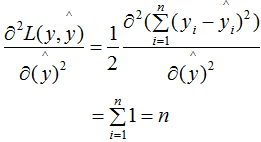
Thus, in the linear regression model, the number of samples at the node represents the sum of instance weights.

2.2 Tree Model

In the tree model, the Hessian represents the instance weights. The condition for whether to split a node is to compare the sum of instance weights at that node with min_child_weight; if greater, it splits; otherwise, it does not split (assuming other conditions for splitting are met).

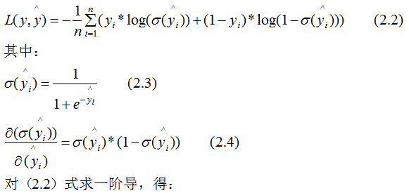
To deepen understanding, this section uses binary logistic regression as an example:

The loss function of binary logistic regression:

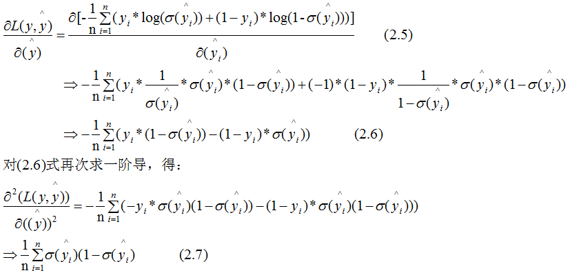
(2.7) represents the sum of instance weights at the node, which can qualitatively show the relationship between (2.7) and min_child_weight:

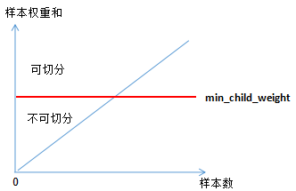
From the above figure, it can be seen that the number of samples is positively correlated with the instance weights, thus the sum of instance weights in the tree model reflects the number of samples to some extent.

From the properties of the XGBoost algorithm, we know:

(1) When yi is 1,the larger it is, the smaller the loss function becomes, and (2.7) approaches 0.

(2) When yi is 0,the smaller it is, the smaller the loss function becomes, and (2.7) approaches 0.

Thus, (2.7) can also represent the purity of a node; if the purity is greater than min_child_weight, the node can continue to split; if the purity is less than min_child_weight, it does not split.

3. Weight Quantile Algorithm

Sort the second derivative of the loss function and then split based on quantiles, selecting the best split point. This will not be expanded here; please refer to the XGBoost split point algorithm for specific details.

4. Conclusion

The XGBoost algorithm uses the second derivative of the loss function (Hessian) to represent instance weights. This concept reflects the number of samples at the node in linear regression models and the purity of the node in tree models.

References: https://stats.stackexchange.com/questions/317073/explanation-of-min-child-weight-in-xgboost-algorithm#

Recommended Reading

Summary of XGBoost Algorithm Principles

XGBoost Split Point Algorithm

Summary of XGBoost Parameter Tuning