
Author: Yishui Hancheng, CSDN Blog Expert, Research Directions: Machine Learning, Deep Learning, NLP, CV
Blog: http://yishuihancheng.blog.csdn.net
This article mainly practices multivariate sequence prediction based on LSTM (Long Short-Term Memory) neural networks, completing the prediction, analysis, and visualization of data at specified future time steps, and teaches you step by step how to build your own predictive analysis model.
The article is divided into three parts: Introduction to the LSTM model, Data Exploration and Analysis, and Model Construction and Testing.
1. Introduction to LSTM Model
Since we are talking about LSTM, we should briefly introduce RNN (Recurrent Neural Network). The LSTM neural network model can be regarded as a type of RNN. RNNs are a class of neural networks specifically designed to process sequential data samples. Each layer not only outputs to the next layer but also outputs a hidden state for use by the current layer when processing the next sample.
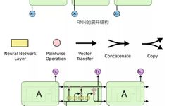
RNNs can infer current information based on previously encountered information, especially in language processing, where RNNs can be used to predict the next word based on the context. However, it can only handle information at certain intervals; if the gap in the context is too far, it may become difficult to relate. This is where LSTM comes into play. The main difference in the unfolded structure of LSTM compared to RNN is the existence of structures that control the storage state. The following figure shows a schematic diagram of the classic RNN model and LSTM model:

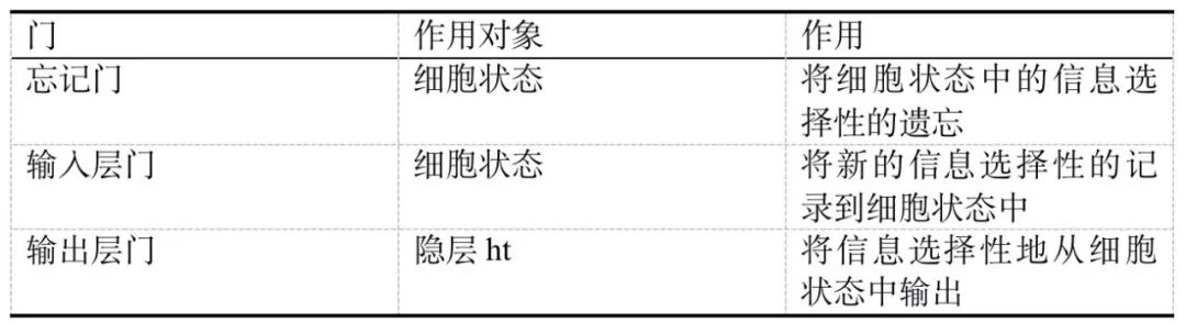
To deeply understand the mechanism of LSTM, it is crucial to clarify the three gates within LSTM. The LSTM model mainly includes: the forget gate, the input gate, and the output gate. A simple introduction to each gate is shown in the table below:
This concludes the detailed introduction of the LSTM model’s principles. To fully grasp its operational mechanisms, one needs to spend some time digesting and understanding it.
Today, this article mainly utilizes the LSTM deep learning model to model and analyze the time series data at hand, constructing our sequence data prediction model to perform multi-step future predictions.
2. Data Exploration and Analysis
The dataset we use here comes from the monitoring data of six conventional atmospheric factors publicly available from a central monitoring station. A partial screenshot of the dataset is shown below:
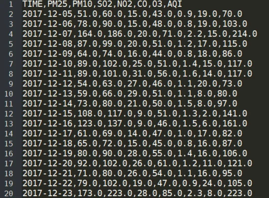
Where TIME, PM25, PM10, SO2, NO2, CO, O3, and AQI represent: monitoring time, PM2.5, PM10, SO2, NO2, CO, O3, and air quality index respectively.
To perform a simple data exploration analysis on the existing dataset, some necessary statistical calculations and visualization analyses are indispensable. Here, I recommend a data overview analysis tool called pandas_profile, which, as the name suggests, is a data overview analysis tool developed based on pandas, and is very convenient to use. Below, we will perform data exploration based on this module, with very little code as follows:
#encoding:utf-8
import pandas as pd
import pandas_profiling
df = pd.read_csv('dataset.csv')
profile=pandas_profiling.ProfileReport(df)
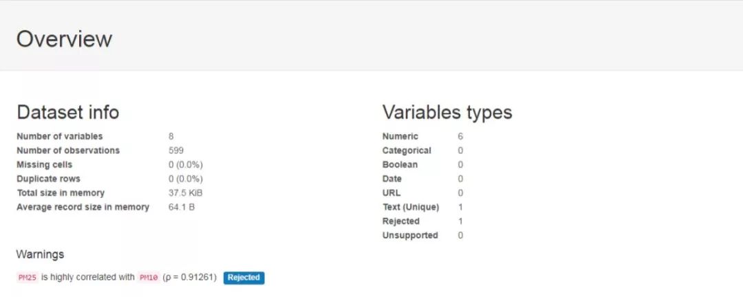
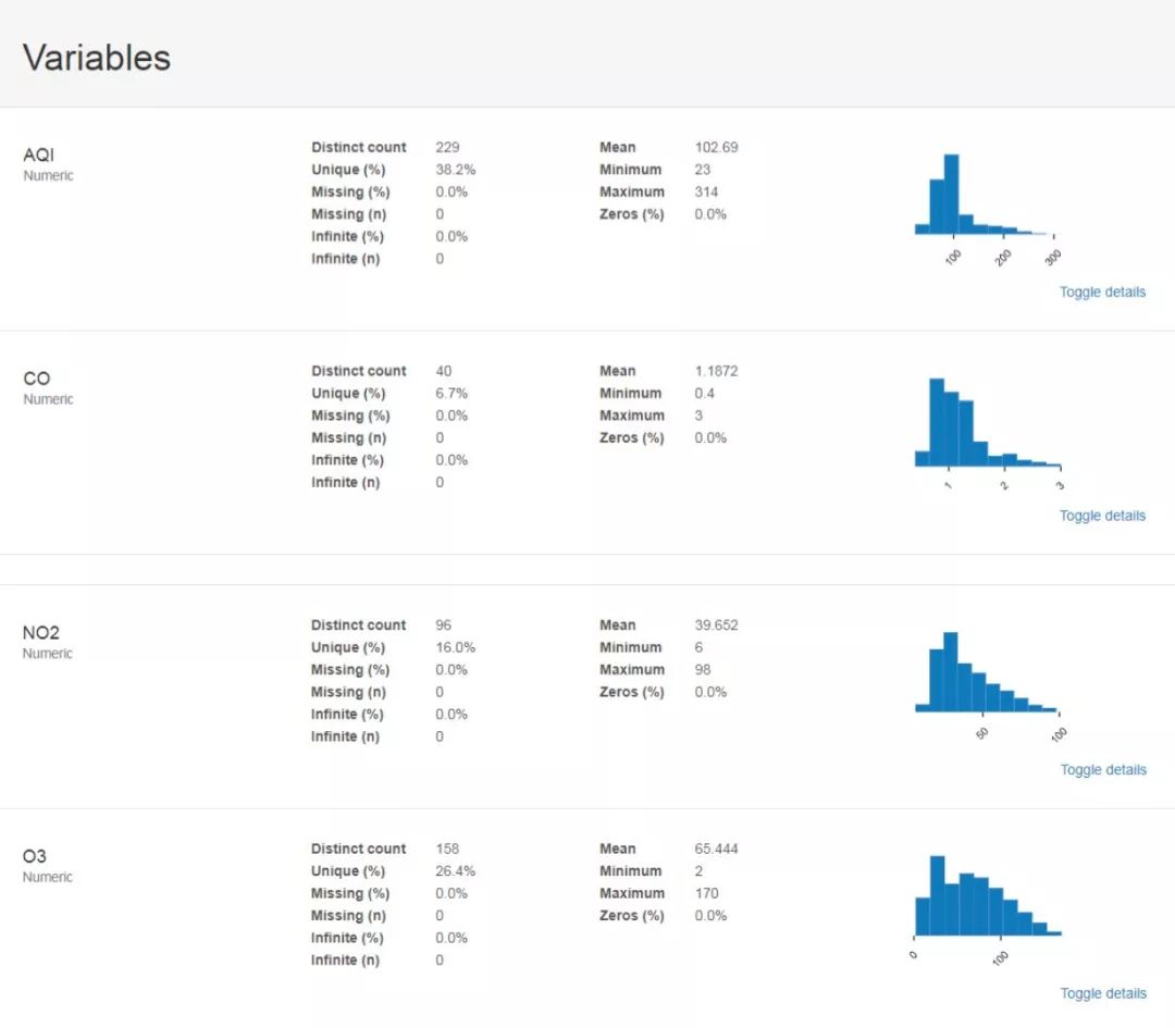
profile.to_file('dataset.html')After running, the relevant analysis results we need have been stored in the local dataset.html, and a screenshot of the content is shown below. First is the overall overview of the dataset and the statistical calculations and distribution results of each factor:

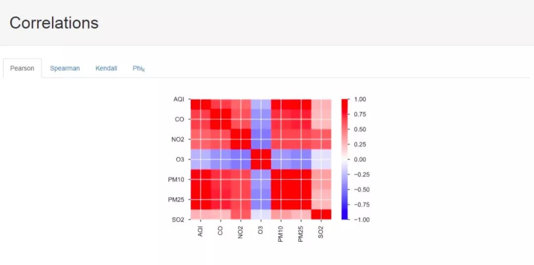
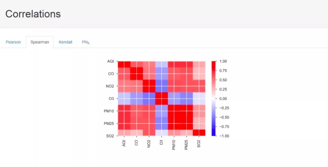
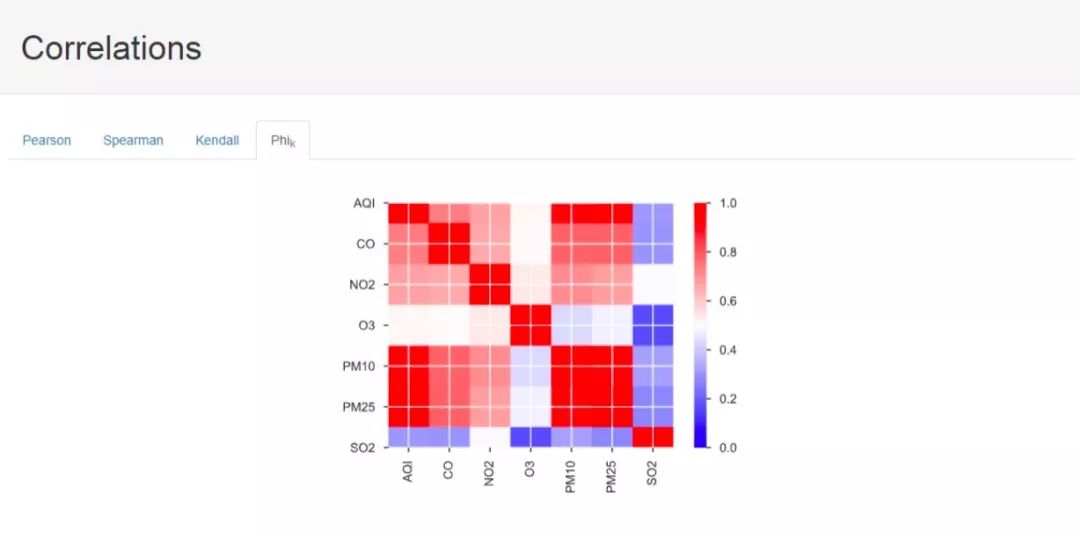
Next is the factor correlation calculation results, where we provide analysis results obtained under four different calculation methods. The first three are the three statistical correlation measures, and the last one I am not sure what algorithm it is. I hope knowledgeable individuals can provide guidance, much appreciated.

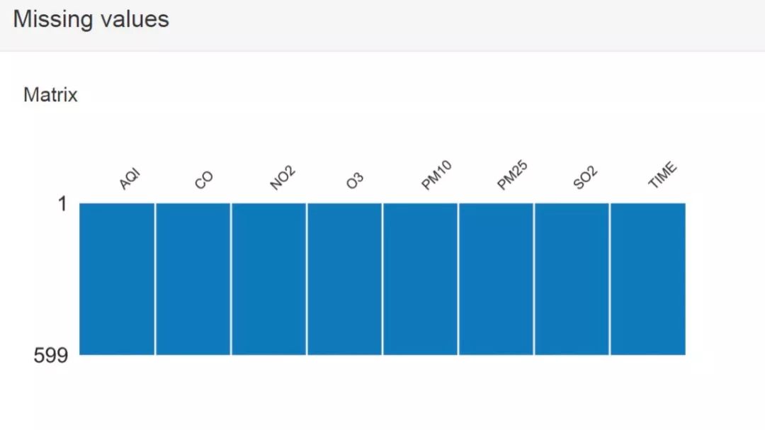
Next, we have information on missing values:

After completing the above data overview analysis, to visualize the trend of different factors more intuitively, we performed visualization analysis based on interactive visualization methods. The data screenshots are shown below:
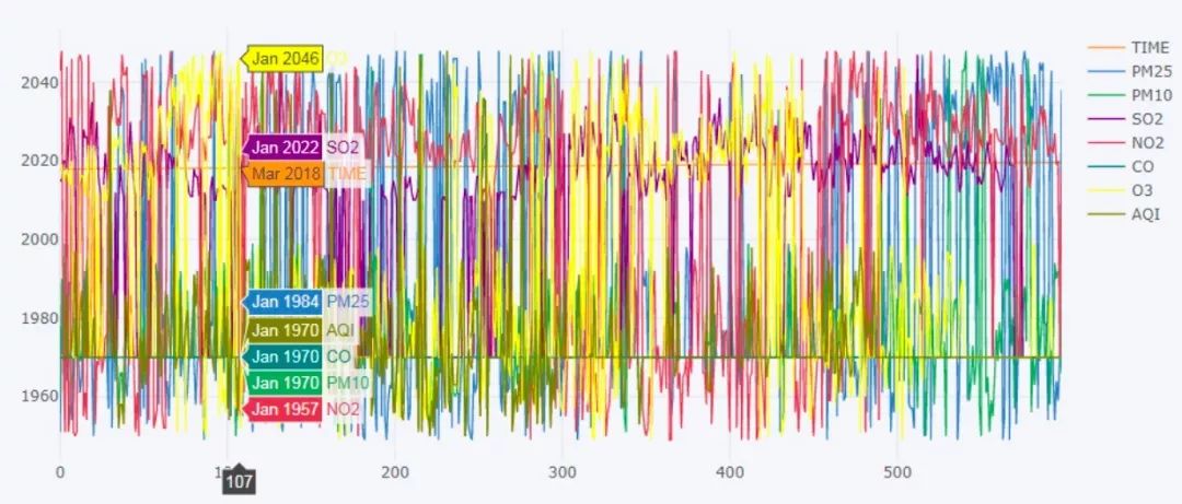
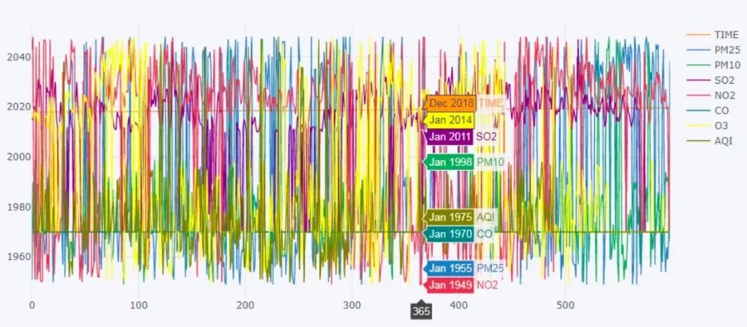
I personally feel that this interactive visualization display method is better than the static display form of matplotlib.
Here, our data exploration and analysis is roughly finished. I want to say that every step is essential in completing the entire machine learning or deep learning process. Data exploration analysis helps us grasp the statistical distribution characteristics of different factors in the dataset, while data visualization analysis can help us discover the overall trends and anomalies in the dataset.
3. Model Construction and Testing
Next, we enter the core practical section: model building. The model building is mainly divided into several steps:
1. Moving sliding window dataset construction 2. Training set and test set splitting 3. Model construction 4. Multi-step sequence rolling prediction function implementation 5. Result data visualization.
Now, we will explain and introduce the five steps one by one:
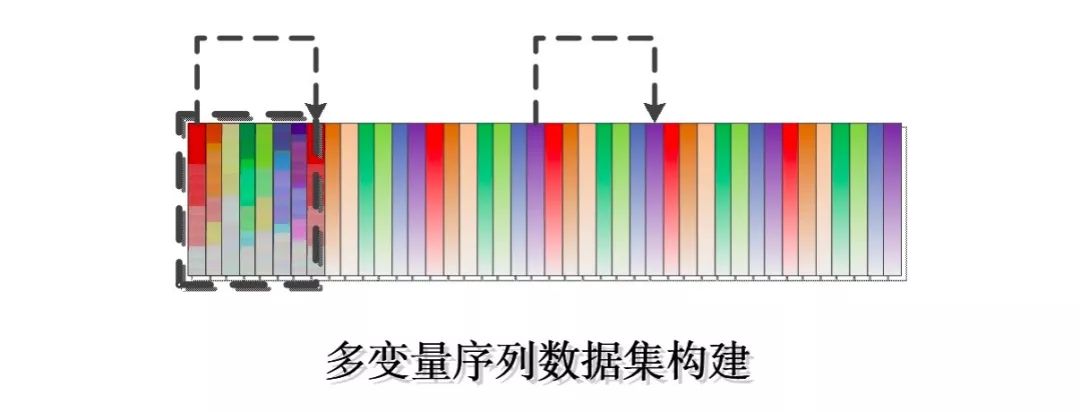
1. Moving Sliding Window Dataset Construction
To predict values for time series data, constructing the dataset is a crucial step. We need to build a supervised dataset based on the original dataset so that our model can learn the characteristics of the original time series data, thus achieving predictions for future time steps. The principle of sliding window dataset construction is shown in the following illustration:
The specific implementation is as follows:
1.def sliceWindow(data,step):
2.    '''''
3.    Create dataset using moving sliding window
4.    '''
5.    X,y=[],[]
6.    for i in range(0,len(data)-step,1):
7.        end=i+step
8.        oneX,oney=data[i:end,:],data[end, :]
9.        X.append(oneX)
10.        y.append(oney)
11.    return np.array(X),np.array(y)
The above 10 lines of code implement the creation of the required dataset.
2. Training Set and Test Set Splitting
In the training process of a supervised model, we will divide the original dataset to obtain the training dataset and test dataset, where the training dataset is used for model training, and the test dataset is used for model evaluation and testing. Here, we do not use the dataset splitting function train_test_split from sklearn mainly because we want to perform time series data prediction analysis, and train_test_split randomly splits the original dataset, which does not preserve the time series nature of the original dataset. This is also a key difference between time series data prediction and other data value predictions. The specific implementation of our dataset splitting is as follows:
1.def dataSplit(dataset,step,ratio=0.70):
2.    '''''
3.    Dataset splitting
4.    '''
5.    datasetX,datasetY=sliceWindow(dataset,step)
6.    train_size=int(len(datasetX)*ratio)
7.    X_train,y_train=datasetX[0:train_size,:],datasetY[0:train_size,:]
8.    X_test,y_test=datasetX[train_size:len(datasetX),:],datasetY[train_size:len(datasetX),:]
9.    X_train=X_train.reshape(X_train.shape[0],step,-1)
10.    X_test=X_test.reshape(X_test.shape[0],step,-1)
11.    print('X_train.shape: ',X_train.shape)
12.    print('X_test.shape: ',X_test.shape)
13.    print('y_train.shape: ',y_train.shape)
14.    print('y_test.shape: ',y_test.shape)
15.    return X_train,X_test,y_train,y_test
Here, ratio represents the proportion of the training dataset.
3. Model Construction
Since Keras was introduced, building deep learning models has become very easy. Here, we implemented the LSTM model construction based on Keras, with the specific implementation as follows:
1.def seq2seqModel(X,step):
2.    '''''
3.    Sequence to sequence stacked LSTM model
4.    '''
5.    model=Sequential()
6.    model.add(LSTM(256, activation='relu', return_sequences=True,input_shape=(step,X.shape[2])))
7.    model.add(LSTM(256, activation='relu'))
8.    model.add(Dense(X.shape[2]))
9.    model.compile(optimizer='adam', loss='mse')
10.    return model
As can be seen above, the model construction is simplified. We specifically separated the model construction into a standalone function, mainly considering decoupling. When the model needs to be modified, there is no need to change the overall functionality; this function can be handled separately, and it is very simple to add a new model function as well.
For example, we also implemented a bidirectional LSTM neural network model based on Keras as follows:
1.def bidirectionalModel(X,step):
2.    '''''
3.    Bidirectional LSTM model
4.    For certain sequence prediction problems, allowing the LSTM model to learn both forward and backward input sequences and connect both interpretations is beneficial.
5.    This is called a bidirectional LSTM, which can be implemented for univariate time series prediction by wrapping the first hidden layer in a layer called bidirectional.
6.    '''
7.    model=Sequential()
8.    model.add(Bidirectional(LSTM(256,activation='relu'),input_shape=(step,X.shape[2])))
9.    model.add(Dense(X.shape[2]))
10.    model.compile(optimizer='adam',loss='mse')
11.    return model
The number of hidden layers and the number of hidden units can be adjusted according to your actual needs.
4. Multi-Step Sequence Rolling Prediction Function Implementation
Many blog articles discuss LSTM time series predictions, but many only focus on single-step predictions. In practical situations, we often need to predict data over a future period, which is what we commonly refer to as a multi-step prediction model. Here, we also implemented a multi-step prediction function as follows:
1.def predictFuture(model,dataset,features,step,next_num):
2.    '''''
3.    Predict future multi-step values
4.    '''
5.    lastOne=(dataset[len(dataset)-step:len(dataset)]).reshape(-1,features)
6.    backData=lastOne.tolist()
7.    next_predicted_list=[]
8.    for i in range(next_num):
9.        one_next=backData[len(backData)-step:]
10.        one_next=np.array(one_next).reshape(1,step,features)
11.        next_predicted=model.predict([one_next])
12.        next_predicted_list.append(next_predicted[0].tolist())
13.        backData.append(next_predicted[0])
14.    return next_predicted_list
Consistent with the model construction approach, we decompose individual functions into independent processing functions, facilitating later modifications and additions of functionalities.
5. Result Data Visualization
Result data visualization is also a very important aspect. We analyze the model’s performance through the degree of fit and trends between predicted data and real data. The code for visualization analysis is as follows:
1.def dataCruvePloter(data_list,future_list,save_path='dataCruvePloter.png'):
2.    '''''
3.    Result curve visualization
4.    '''
5.    plt.clf()
6.    plt.figure(figsize=(20,12))
7.    factor=['PM25','PM10','SO2','NO2','CO','O3','AQI']
8.    dataset=[]
9.    for i in range(len(data_list)):
10.        dataset.append([float(O) for O in data_list[i][1:]])
11.    for j in range(7):
12.        D1,D2=[one[j] for one in dataset],[one[j] for one in future_list]
13.        plt.subplot(2,4,j+1)
14.        plt.plot(list(range(len(D1))),D1,label=factor[j]+' True')
15.        plt.plot(list(range(len(D1),len(D1)+len(D2))),D2,label=factor[j]+' Predict')
16.        plt.legend(loc='best',ncol=2)
17.    plt.savefig(save_path)
After completing all five steps, we can now call our model for training, prediction, and analysis. The code implementation is as follows:
1.#Dataset loading
2.with open('dataset.txt') as f:
3.    data_list=[one.strip().split(',') for one in f.readlines()[1:] if one]
4.dataset=[]
5.for i in range(len(data_list)):
6.    dataset.append([float(O) for O in data_list[i][1:]])
7.dataset=np.array(dataset)
8.step=7
9.X_train,X_test,y_train,y_test=dataSplit(dataset,step)
10.#model=bidirectionalModel(X_train,step)
11.model=seq2seqModel(X_train,step)
12.model.fit(X_train,y_train,epochs=50,verbose=0)
13.#Model testing sample
14.test=[
15.      [30.0,58.0,7.0,24.0,0.9,83.0,103.0],
16.      [43.0,72.0,6.0,23.0,1.1,85.0,103.0],
17.      [66.0,105.0,6.0,22.0,1.3,134.0,103.0],
18.      [54.0,94.0,7.0,27.0,1.1,125.0,103.0],
19.      [64.0,90.0,6.0,19.0,1.2,127.0,103.0],
20.      [59.0,92.0,6.0,20.0,1.1,126.0,103.0],
21.      [61.5,91.0,6.0,19.5,1.15,134.0,103.0]
22.     ]
23.#True value   [38.0,66.0,5.0,17.0,1.2,138.0,103.0]
24.test=np.array(test)
25.test=test.reshape((1,step,7))
26.y_pre=model.predict(test,verbose=0)
27.print('y_pre: ',y_pre)
28.future_list=predictFuture(model,dataset,7,step,60)
29.dataCruvePloter(data_list,future_list,save_path='dataCruvePloter.png')
The result output is as follows:
1.y_pre: [40.86961,65.5033,4.8647,30.08823,1.16613,136.06862,100.5173]In my previous blog post, I wrote about the evaluation metrics for regression models. Here, I will share it again. If you need to calculate the corresponding metrics to evaluate model performance, you can use the following implementation:
1.#!usr/bin/env python
2.#encoding:utf-8
3.from __future__ import division
4.
5.
6.''''
7.__Author__: Yishui Hancheng
8.Function: Calculate four common evaluation metrics in regression analysis models
9.'''
10.
11.from sklearn.metrics import explained_variance_score, mean_absolute_error, mean_squared_error, r2_score
12.
13.
14.
15.def calPerformance(y_true,y_pred):
16.    '''''
17.    Model effect metrics evaluation
18.    y_true: True data values
19.    y_pred: Predicted data values from regression model
20.    explained_variance_score: The variance score of the regression model, which ranges from [0,1]. The closer to 1, the more the independent variable can explain the variance change of the dependent variable.
21.    The smaller the value, the worse the effect.
22.    mean_absolute_error: Mean Absolute Error (MAE), used to assess the closeness of predicted results to the true dataset. The smaller the value, the better the fitting effect.
23.    mean_squared_error: Mean Squared Error (MSE), this metric calculates the mean of the squared errors between the fitted data and the original data corresponding sample points. The smaller the value, the better the fitting effect.
24.    r2_score: Coefficient of determination, which also explains the variance score of the regression model. Its value ranges from [0,1]. The closer to 1, the more the independent variable can explain the variance change of the dependent variable. The smaller the value, the worse the effect.
25.    '''
26.    model_metrics_name=[explained_variance_score, mean_absolute_error, mean_squared_error, r2_score]
27.    tmp_list=[]
28.    for one in model_metrics_name:
29.        tmp_score=one(y_true,y_pred)
30.        tmp_list.append(tmp_score)
31.    print ['explained_variance_score','mean_absolute_error','mean_squared_error','r2_score']
32.    print tmp_list
33.    return tmp_list
34.
35.
36.if __name__=='__main__':
37.    y_pred=[22, 21, 21, 21, 22, 26, 28, 28, 33, 41, 93, 112, 119, 132, 126]
38.    y_true=[23, 23, 23, 22, 23, 26, 28, 28, 32, 37, 56, 64, 68, 74, 75]
39.    calPerformance(y_true,y_pred)
The visualization analysis curve of the model prediction results is shown below:
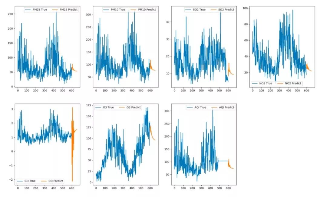
In summary, regarding the business background and prediction results: the prediction of CO showed negative values, which is incorrect and may be related to the data volume in the model. After all, our dataset only contains a few hundred records, which is quite insufficient for deep learning models. Today, our work mainly involved the complete practice of the LSTM multivariate multi-step sequence prediction model, teaching you step by step how to build your own predictive analysis model.
If you are interested, you can take the code we provided to try it out and familiarize yourself with the entire modeling and processing analysis process.
Appreciate the Author

The Python Chinese Community, as a decentralized global technical community, aims to become a spiritual tribe of 200,000 Python Chinese developers. It currently covers major media and collaboration platforms, establishing extensive connections with well-known companies and technical communities in the industry, including Alibaba, Tencent, Baidu, Microsoft, Amazon, Open Source China, CSDN, and more. It has tens of thousands of registered members from more than ten countries and regions, including government agencies, research institutions, financial institutions, and well-known companies at home and abroad, represented by the Ministry of Public Security, Ministry of Industry and Information Technology, Tsinghua University, Peking University, Beijing University of Posts and Telecommunications, People’s Bank of China, Chinese Academy of Sciences, CICC, Huawei, BAT, Google, Microsoft, etc., with nearly 200,000 developers following across all platforms.
2019 Global Mobile Developer Technology Summit
Send Limited Time Free Tickets 50 Tickets


(Scan to register – click free ticket – fill in invitation code:Python Chinese Community– submit for review)