
Transcription | Li Sijie
1. Background: Multi-Hop Reasoning on Knowledge Graphs?
(1) Knowledge Graph
The concept of knowledge graphs was proposed around 1970, and by around 2000, Google began to develop this concept as a key area.
Knowledge graphs originate from graphs, consisting of a set of nodes and edges, where each node and edge is filled with entities, giving it specific meanings, which is the essence of knowledge graphs.
The following image shows four common knowledge graphs. The first is the open-page knowledge graph, such as Wikipedia; the second is the currently popular domain training, such as ChatGPT; the third is related to COVID-19 research, which may also be prevalent in the next 5-10 years; the fourth is social networks, where influence, followers, connections, and regions can all be constructed into corresponding knowledge graphs.
In the development of knowledge graphs over the past thirty to forty years, there have been many applications and implementations that have achieved certain effects, but no milestone developments have emerged. Therefore, it remains to be seen how to truly maximize the potential of knowledge graphs. There are still many issues within knowledge graphs, including entity alignment, knowledge graph cleaning, and how to create segmented vertical domains, all of which are relatively complex problems that still need resolution.
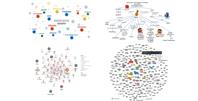
Figure 1 Knowledge Graph
(2) Objective
Our objective is to perform multi-hop reasoning on knowledge graphs, specifically to construct edges for nodes, then map queries to the knowledge graph, and finally find the last node through the knowledge graph, which is our answer.
In multi-hop logical reasoning on knowledge graphs, a traditional approach for path searching is TransE, which has many related variant models. For spatial embedding, it has two branches: one for shape embedding and the other for probabilistic embedding, such as BETAE, GammaE, and GaussianE.
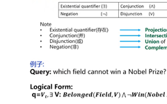
(3) First-order Logical Queries (FOL)
First-order logical queries refer to extracting corresponding entities from the query during task execution. In the example below, ‘field’ and ‘Nobel Prize’ are the corresponding entities, while ‘cannot win’ is the relationship, and the entities and relationships can be transformed into corresponding logical forms. In logical forms, basic logical operations performed by the computer are substituted, including the following four operations: Existential quantifier, Conjunction, Disjunction, and Negation, which can construct logical forms.
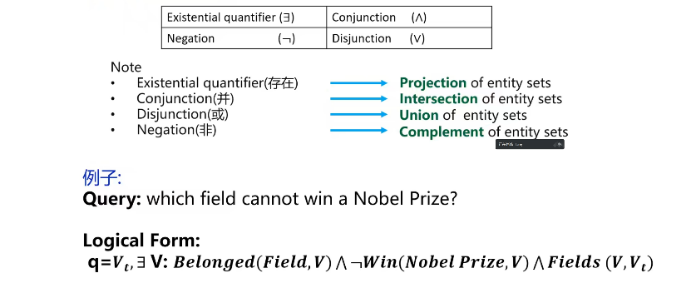
Figure 2 First-order Logical Queries
The following diagram illustrates the most basic logical units in logical multi-hop reasoning, including single-hop questions, long-path questions, conjunction questions, disjunction questions, and negation questions.
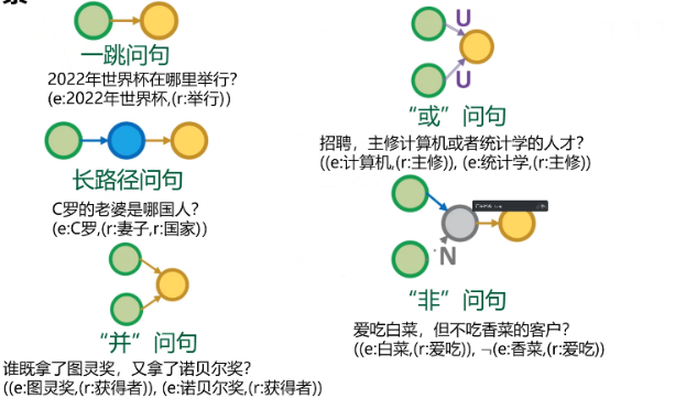
Figure 3 Basic Logical Units
(4) Path Search: TransE
So how do we calculate with these logical units? The initial method is TransE, which maps all entities (head entity and tail entity) and relationships to a low-dimensional vector space. Multi-hop reasoning starts with the head entity h, adding n steps of relationships r, step by step to the corresponding query.
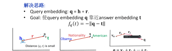
Figure 4 Path Search: TransE
The advantage of TransE is that it can handle any triplet relationships and logical operations, but it also has drawbacks. First, due to the incompleteness of knowledge graphs, some entities cannot be found through traversal, resulting in poor convergence during training and decreased performance. Second, the high computational cost. During multi-hop reasoning, all intermediate head and tail entities must be recorded, leading to significant overhead and decreased timeliness.
2. Models
To address these issues, spatial models have been proposed. The best method for spatial embedding models is that they do not need to record these intermediate entities; only the final query embedding needs to be calculated.
(1) BETAE
The first model is BETAE. As shown in the calculation graph, all entities are first mapped into the corresponding BETA distribution, abstracting them into a BETA space, initializing α and β. A key point is that both α and β can be constructed multidimensionally; we constructed 800-dimensional matched pairs of α and β for processing, where each entity has basic logical operations.
Advantages: BETAE can directly perform projection, intersection, and negation operators.
Disadvantages: To perform the union operator, BETAE requires the use of De Morgan’s laws (DM) and disjunctive normal form (DNF).
In BETAE, the initial embedding and its complementary embedding always have two intersection points, which may lead to boundary issues.

Figure 5 BETAE
Next, we introduce disjunctive normal form (DNF). As shown on the left, there are three entities corresponding to query embeddings, performing spatial embedding for each node, where two nodes use union (OR) logical operation. However, when introducing a fourth node, performing a union on v2, v3, and v4 in the BETA distribution will include v3, which is not what we want. We can perform the union across the entire space, rather than in a closed environment, which is the method of disjunctive normal form.
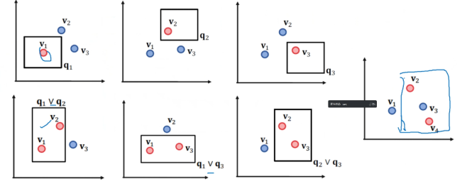
Figure 6 Disjunctive Normal Form
In the calculation graph, the union is removed from the first step and moved to the last, replacing each previous step with projection and intersection, and finally calculating the union. The steps are as follows:
1. Take one end of all union operators as the parent node.
2. Remove all union operators, keeping the parent node.
3. Split the target sink nodes of each calculation graph, which are the nodes that aggregate calculation results, allowing each calculation graph to perform joint calculations.
4. Generate new sink nodes, aggregating the results of each calculation graph into the sink node.
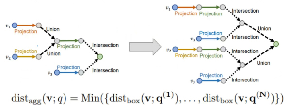
Figure 7 Disjunctive Normal Form
Next is the model design of BETAE. During testing, it primarily performs logical multi-hop reasoning, which can be split into the most basic computational logical units. As shown in the figure, we can see that during testing, it generally produces the best results, and the effect of using DNF for union is significantly better than DM. This is because DNF handles the previous unions with intersections and negations, and when performing the final union, it seeks the minimum distance, compressing the space, resulting in outcomes closer to actual results.
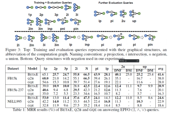
Figure 8 BETAE Model Design
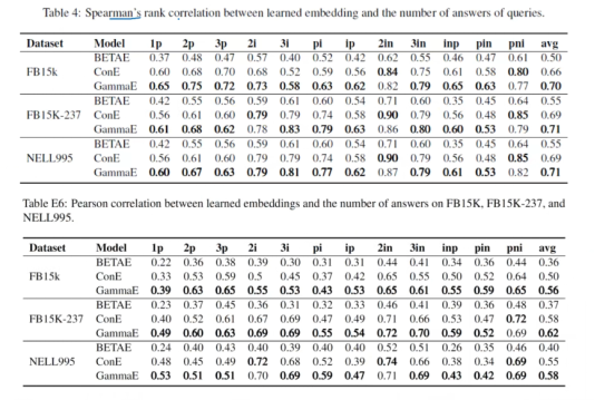
Next, we compute the similarity against Spearman, calculating the similarity between the learned query embedding and the actual answer embedding, which also yields very good overall results. Table 4 shows the ROC and AUC for the training of BETA, indicating that its ROC and AUC are very high, demonstrating the model’s robustness. Its intersection performs well, while projection performs slightly less.
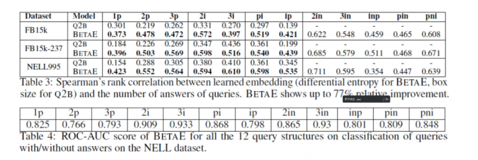 Figure 9 BETAE Model Design
(2) GammaE
The second model is GammaE.
GammaE has a distribution similar to BETAE, also initializing α and β; however, what are the advantages of Gamma distribution over BETA distribution? Gamma distribution also has four basic logical operations (projection, intersection, union, negation), where the projection operator and intersection operator are quite similar to the previous ones.
Its innovation comes from the union operator and negation operator. The first innovation is that the union uses a gamma mixture model, accumulating weights for each; the second innovation introduces elasticity, slightly adjusting the entire embedding upward, which is the core innovation of this paper. Its advantage is that α and β are directly calculated through formulas, which is essentially lossless and significantly speeds up computations. GammaE effectively avoids DM and DNF, requiring only simple multiplication of all distributions and summing weights.
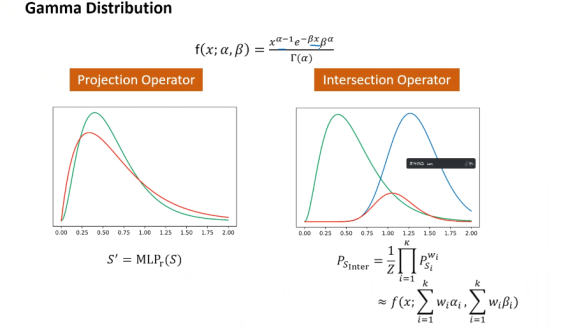
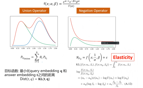
Figure 10 GammaE
The following image illustrates an example from the paper. The upper part shows a normal calculation graph, while the lower part shows the mapping of Gamma in two-dimensional space, where the final answer found is ‘mathematics’ instead of ‘physics’.
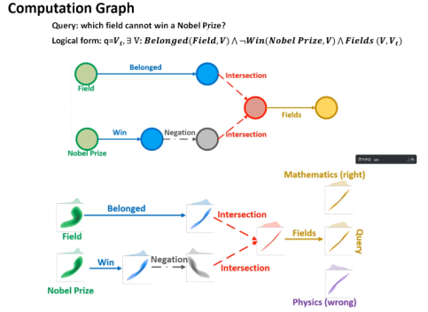
Figure 11 GammaE Example
In the experimental setup, GammaE is essentially similar to the previous BETAE, with corresponding experimental design details.
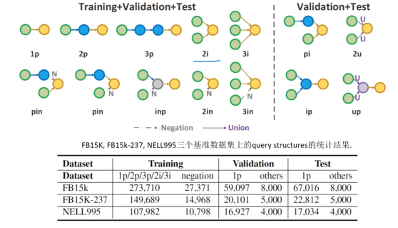
Figure 12 Experimental Setup
In the EPF0 question, Table 1 shows that GammaE improves MRR by an average of 5.0%, 3.8%, and 3.7% over the previously best-performing ConE on FB15k, FB15k-237, and NELL995, respectively.
Table 2 shows that GammaE significantly improves baseline performance by 17.2%, 23.9%, and 25.8% on FB15k, FB15k-237, and NELL995.
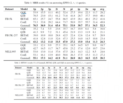
Figure 13 Experimental Results: EPF0 Question
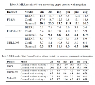
In the negation question, GammaE achieves an average MRR increase of 12.2%, 14.9%, and 9.1% over the two baselines on FB15k, FB15K-237, and NELL995.
The elasticity ε can significantly enhance the performance of GammaE.
In terms of model robustness, GammaE outperforms all previous models, with correlations on B15k, FB15k-237, and NELL995 exceeding ConE by 6.1%, 2.9%, and 2.9%, respectively. GammaE can effectively reduce the uncertainty of queries.
In conjunction questions, GammaE using a mixture model (MM) outperforms GammaE using De Morgan’s laws (DM) and disjunctive normal form (DNF).
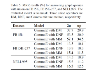
Figure 16 Analysis: Conjunction Question
(3) GaussianE
The third model is GaussianE. Compared to the previous two works, this work is also open-source, but it has bugs in the code; nonetheless, its overall approach is still quite inspiring.
In knowledge graph embedding, it performs a simple mapping of entities and relationships, and during this process, the entire shape changes after performing union operations, no longer resembling a box. Gaussian embedding effectively addresses this issue. As shown in the right image, after performing union, it remains close to a Gaussian distribution space, and GaussianE represents this well through a Gaussian mixture model, which is a good solution.
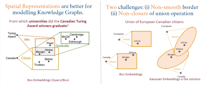
Figure 17 GaussianE
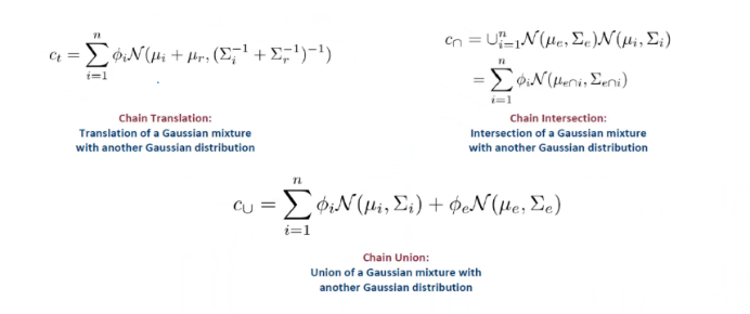
Multivariate Gaussian Representations solve the following issues: First, capturing spatial features of entities and relationships. Second, smoothing boundaries through Mahalanobis distance, maintaining the original spatial shape after performing unions. Third, closing union operations through Gaussian mixtures. Fourth, achieving scalability through chain reasoning. It also effectively avoids Morgan’s laws (DM) and disjunctive normal form (DNF).
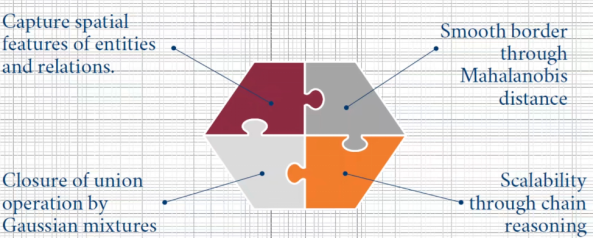
Figure 18 Problems Solved by GaussianE
GaussianE introduces a distance measure. Previously, the spatial distance in models was a simple Euclidean distance; here, it is Mahalanobis distance. This is inherently present in the Multivariate Gaussian mixture model, meaning it is a natural choice for smoothing distance functions in multivariate Gaussian mixtures. As shown in the left image, during the union of boxes, Hinton is placed in the middle due to both being present and not enclosed by the box. In the right image, the Gaussian distribution can effectively encompass him, and its entire curve is also very smooth. Additionally, the overall distance calculation is significantly smaller and more precise.
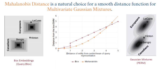
Figure 19 GaussianE Example 1
As shown in the table below, Bengio has the shortest distance in Canadian, and LeCun has the shortest distance in European; these are objective facts that are all included, and their distances using Gaussian Mixture and union of boxes operations are also close. Hinton is also included, but in the union of boxes, the distance is large, so he is not included. After using Mahalanobis distance, his distance significantly decreases, allowing him to be included, effectively selecting the Hinton entity.
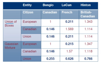
Figure 20 GaussianE Example 1
Previous models were projection-based, meaning they existed. The following demonstrates the Translation, Intersection, and Union queries of GaussianE.
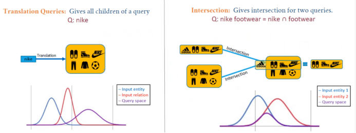
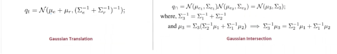
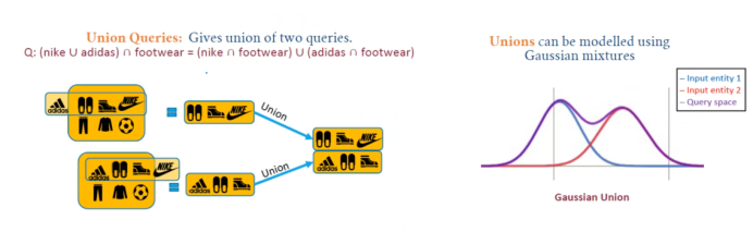
Figure 21 GaussianE Example 2
Finally, there are multiple entities; these formulas also exist and can be applied. However, the intersection and union they compute are very close, which is a significant drawback.
Advantages of GaussianE include:
1. Single Gaussian/Box query operations require very little memory.
2. Gaussian operations are closed under Gaussian mixture models, whereas boxes are not.
3. Box operations require disjunctive normal form (DNF) transformation during union operations (requiring the entire query). Therefore, long queries cannot be simplified into individual operations; Gaussian queries can be simplified into single query operations and can be merged through continuous chain operations. Thus, they can be applied to queries of any length.
The following is a comparison of the overall performance of the models. GaussianE embedding shows a significant improvement over previous models, performing the best across all four datasets, achieving optimal results overall.
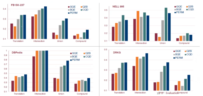
Figure 23 GaussianE Performance
3. Conclusion
1. We introduced a new logical reasoning model, namely BETAE, GammaE, and GaussianE, to handle arbitrary FOL queries and effectively implement multi-hop reasoning on KG.
2. Detailed the design and principles of each model.
3. Through extensive experimental results, showcased the strengths and weaknesses as well as performance of these models.
   ABOUT
    About Us
Deep Blue Academy, incubated at the Institute of Automation, Chinese Academy of Sciences, is an online education platform focused on artificial intelligence, robotics, and autonomous driving, with over 100,000 students learning on the Deep Blue Academy platform, many from well-known universities both domestically and internationally, such as Tsinghua and Peking University, aiming to cultivate cutting-edge technical talents usable by enterprises.