Abstract

arXiv:2310.08278v3 [cs.LG] February 8, 2024

Original paper link: https://arxiv.org/pdf/2310.08278

In recent years, foundation models have caused a paradigm shift in the field of machine learning due to their unprecedented zero-shot and few-shot generalization capabilities. However, despite the success of foundation models in fields such as natural language processing and computer vision, the development of foundation models for time series forecasting has lagged behind. We propose Lag-Llama, a general foundation model for univariate probabilistic time series forecasting based on a decoder-only transformer architecture, utilizing lags as covariates. Lag-Llama has been pre-trained on a large corpus of diverse time series data from multiple domains and has been compared with various forecasting models on zero-shot generalization capabilities across downstream datasets. Moreover, when fine-tuned on relatively small unseen datasets, Lag-Llama achieves state-of-the-art performance, outperforming previous deep learning methods on average, establishing itself as the best general model. Lag-Llama is a strong contender in the field of time series forecasting and paves the way for further development of foundation models targeting time series data.

Introduction

Probabilistic time series forecasting is an important practical problem involving various application domains, from finance and weather forecasting to brain imaging and computer system performance management (Peterson, 2017). Accurate probabilistic predictions are often a crucial step for subsequent decision-making in these practical areas. The probabilistic nature of such predictions provides decision-makers with a concept of uncertainty, allowing them to consider various future scenarios and their corresponding probabilities. Various methods have been proposed to tackle this issue, ranging from classic autoregressive models (Hyndman & Athanasopoulos, 2021) to state-of-the-art neural forecasting methods based on deep learning architectures (Torres et al., 2021). It is worth noting that the vast majority of these previous methods focus on building models specific to particular datasets, i.e., models tested on the same dataset on which they were trained.

However, recently, the field of machine learning has been undergoing a paradigm shift due to the rise of foundation models (Bommasani et al., 2022)—large-scale, general neural networks pre-trained in an unsupervised manner across various data distributions. These models have demonstrated extraordinary few-shot generalization capabilities (Brown et al., 2020a), often outperforming models specific to certain datasets. Following the success of foundation models in the domains of language and image processing (OpenAI, 2023; Radford et al., 2021), our goal is to develop a foundation model suitable for time series, investigating its behavior in large-scale scenarios and pushing the achievable transfer limits across different time series domains.

In this paper, we introduce Lag-Llama—a probabilistic time series forecasting foundation model trained on a large corpus of open time series data and evaluated on unseen time series datasets. We investigate the performance of Lag-Llama when encountering unseen time series datasets with different data history levels and demonstrate its performance compared to state-of-the-art models specific to certain datasets.

Our Contributions:

• We propose Lag-Llama, a univariate probabilistic time series forecasting foundation model based on a simple decoder-only transformer architecture that utilizes lags as covariates.

• We demonstrate that Lag-Llama exhibits strong zero-shot performance on unseen datasets when pre-trained from scratch on a broad, diverse corpus of datasets, performing comparably to models trained on specific datasets.

• Lag-Llama showcases state-of-the-art performance on diverse datasets from different domains, becoming the best general model after fine-tuning without prior knowledge of downstream datasets.

• We illustrate Lag-Llama’s strong few-shot adaptation performance on previously unseen datasets, including variations in different data history levels.

• We investigate the diversity of the pre-training corpus used for training Lag-Llama and present the scaling laws of Lag-Llama relative to the pre-training data.

Related Work

Statistical Models are the cornerstone of time series forecasting, continuously evolving to address complex forecasting challenges. Traditional models such as ARIMA (AutoRegressive Integrated Moving Average) lay the groundwork for predicting future values by utilizing autocorrelation. ETS (Error, Trend, Seasonality) models achieve more nuanced predictions by decomposing time series into their fundamental components, capturing trends and seasonal patterns. The Theta model, introduced by Assimakopoulos & Nikolopoulos (2000), is another significant advancement in time series forecasting. By applying a combination of long-term trend and seasonal decomposition techniques, these models provide a simple yet effective forecasting approach. Despite the considerable success of these statistical models and more advanced models (Croston, 1972; Syntetos & Boylan, 2005; Hyndman & Athanasopoulos, 2018), they share common limitations. Their main drawback lies in their inherent assumptions about linear relationships and stationarity in time series data, while real-world scenarios often exhibit abrupt changes and non-linear dynamics. Additionally, they may require extensive manual tuning and specific discrete sets of samples to select appropriate models and parameters for specific forecasting tasks.

Neural Forecasting is a rapidly evolving research area driven by the explosion of machine learning (Benidis et al., 2022). Various architectures have been developed, starting from RNN and LSTM-based models (Salinas et al., 2020; Wen et al., 2018). Recently, given the success of transformers (Vaswani et al., 2017) in sequence-to-sequence modeling for natural language processing, many variants of transformers have been proposed for time series forecasting. Different models (Nie et al., 2023a; Wu et al., 2020a;b) handle input time series in various ways to be understandable by standard transformers, and then reprocess the output of the transformers for point predictions or probabilistic predictions. On the other hand, various other works have proposed alternative attention strategies and built better models for time series based on transformer architectures (Lim et al., 2021; Li et al., 2023; Ashok et al., 2023; Oreshkin et al., 2020a; Zhou et al., 2021a; Wu et al., 2021; Woo et al., 2023; Liu et al., 2022b; Zhou et al., 2022; Liu et al., 2022a; Ni et al., 2023; Li et al., 2019; Gulati et al., 2020).

Foundation Models are an emerging paradigm of self-supervised (or unsupervised) learning, pre-trained on large-scale datasets (Bommasani et al., 2022). Many such models (Devlin et al., 2019; OpenAI, 2023; Chowdhery et al., 2022; Radford et al., 2021; Wang et al., 2022) have demonstrated cross-modal adaptability, extending to scientific domains such as protein design (Robert Verkuil, 2022). The scale of the model, the size of the dataset, and the diversity of the data have also been shown to significantly impact transferability and excellent few-shot learning capabilities (Thrun & Pratt, 1998; Brown et al., 2020b). Self-supervised learning techniques have also been proposed for time series (Li et al., 2023; Woo et al., 2022a; Yeh et al., 2023). The work most relevant to ours is by Yeh et al. (2023), who trained their model on a corpus of time series datasets. The main distinction is that they validated their model only on downstream classification tasks, without validation on forecasting tasks. Works like Time-LLM (Jin et al., 2023), LLM4TS (Chang et al., 2023), GPT2 (Zhou et al., 2023a), UniTime (Liu et al., 2023), and TEMPO (Anonymous, 2024) freeze the backbone of the LLM encoder when fine-tuning/adapting inputs and distribution heads for predictions. The primary goal of our work is to apply foundation model methods to time series data and explore the achievable transfer range across a wide range of time series domains.

Probabilistic Time Series Forecasting

We consider a dataset containing individual univariate time series, sampled at specific discrete time points, where represents the length of the time series. Given this dataset, our goal is to train a forecasting model capable of accurately predicting the future values of the time series over time steps; we refer to these time steps as the test dataset, represented as

The univariate probabilistic time series forecasting problem involves modeling the unknown joint distribution of future values of a one-dimensional sequence, given its observed past up to the time step and covariates:

where represents the parameters of the parameterized distribution. In practice, we can choose to fix the entire historical record of the subsampled time series, which may vary greatly, or opt to subsample it.

When modeling the distribution with a neural network that has parameters, the predictions will be conditioned on these (learned) parameters. We will use autoregressive models to approximate the distribution in formula (2), using the chain rule of probabilities as follows:

## Lag-Llama

We propose Lag-Llama, a foundation model for univariate probabilistic forecasting. The first step in building a foundation model for time series is training it on a large and diverse corpus of time series data. When trained on heterogeneous univariate time series corpora, the frequencies of the time series in our corpus vary. Additionally, when adapting our foundation model to downstream datasets, we may encounter combinations of new and seen frequencies, which our model should be able to handle. We now introduce a general approach for tokenizing series from such datasets without directly relying on the frequencies of any specific dataset, potentially allowing combinations of unseen and seen frequencies to be used at test time.

## Tokenization: Lag Features

The tokenization scheme of Lag-Llama involves constructing “lag features” from previous values of the time series, based on a specified set of appropriate lag indices, including quarterly, monthly, weekly, daily, hourly, and second-level frequencies. Given a set of ordered positive lag indices *L* = {*1*, . . . , *L*}, we define the lag operation to take a specific time value, where each entry of is given as . Therefore, to create lag features for a certain context length window, we need to sample a larger window containing more than points, denoted as . In addition to these lag features, we also add date-time features from all frequencies in our corpus starting from the time index, i.e., from the seconds of minutes, days of hours, etc., up to the quarters of years. Note that while the main goal of these date-time features is to provide additional information, for any time series, all date-time features except one remain unchanged from one time step to the next, which the model can implicitly understand the frequency of the time series. Assuming we used a total of date-time features, our size of each token is . Figure 1 shows an example of tokenization. We note that one drawback of using lag features in tokenization is that it requires a context window size of or larger.

## Lag-Llama Architecture

The architecture of Lag-Llama is based on the decoder-only transformer architecture LLaMA (Touvron et al., 2023). Figure 2 shows a general schematic of the model, which contains M decoder layers. The univariate sequence of length x_{-L: C}^{i} and its covariates are tokenized by concatenating the covariate vector to the C tokens of the sequence 	extbf{x}_{1: C}^{i}. These tokens are passed through a shared linear projection layer, mapping features to the hidden dimension of the attention module. Similar to Touvron et al. (2023), Lag-Llama adopts pre-normalization (RMSNorm) (Zhang & Sennrich, 2019) and rotary position encoding (RoPE) (Su et al., 2021) in the query and key representations of each attention layer, just like in LLaMA (Touvron et al., 2023). After passing through the transformer layers with causal masking, the model predicts the parameters of the predictive distribution for the next time step, where the parameters are output by the parameterized distribution head as described in Section 4.3. The negative log-likelihood of the predictive distributions for all predicted time steps is minimized. During inference, given at least L time series, we can construct a feature vector to pass to the model to obtain the distribution for the next time point. Through greedy autoregressive decoding, we can obtain many simulated trajectories into our chosen prediction horizon P ≥ 1. From these empirical samples, we can compute uncertainty intervals related to downstream decision tasks and metrics associated with the retained data.

## Choice of Distribution Head

The last layer of Lag-Llama is an independent layer called the “distribution head,” which projects the model’s feature representation onto the parameters of a probability distribution. We can combine different distribution heads with the model’s representational capacity to output parameters of any parameterized probability distribution. In our experiments, we adopted the Student *t* distribution as the distribution head and output three parameters corresponding to this distribution, namely degrees of freedom, mean, and standard deviation, ensuring that the appropriate parameters remain positive through suitable nonlinear functions. More expressive distribution choices, such as normalizing flows (Rasul et al., 2021b) and copulas (Salinas et al., 2019a; Drouin et al., 2022; Ashok et al., 2023), are potential distribution head selections but may lead to difficulties in model training and optimization. Our work aims to maintain model simplicity as much as possible, thus opting for a simple parameterized distribution head. Exploration of these distribution heads is left for future work.

## Scaling Values

When training on a large amount of time series data from different datasets and domains, the magnitude of values for each time series may differ. Since we pre-trained a foundation model on these data, we utilized a scaling heuristic (Salinas et al., 2019b), where for each univariate window, we calculate its mean and variance. We can then replace the time series in the window with. We also use and as time-independent real-valued covariates for each token, providing input statistics to the model, which we refer to as summary statistics.

Training Strategies

We adopt a series of training strategies to effectively pre-train Lag-Llama on the dataset corpus. First, we found that adopting a stratified sampling method, where the total number of series in the pre-training corpus is weighted for randomly sampled windows from the pre-training corpus, is useful. Furthermore, we found that employing time series augmentation techniques such as Freq-Mix and Freq-Mask (Chen et al., 2023) helps reduce overfitting. We incorporate hyperparameter search for these augmentation strategies as part of our hyperparameter search.

Experimental Setup

Datasets

We reserved some datasets from each domain to test the few-shot generalization ability of the pre-trained model while using the remaining datasets for pre-training the foundation model. Moreover, we also retained datasets from entirely different domains to evaluate our model’s performance on data that might lack similarity to the pre-training datasets. This setup simulates real-world use cases where one might apply the model to datasets closely related to the domain distribution on which it was trained, as well as to datasets from entirely different domains. Our pre-training corpus contains a total of 7,965 different univariate time series, each varying in length, totaling approximately 352 million data windows (tokens) for our model to train on. Appendix A lists the datasets we used, along with their sources and properties, their respective domains, and the dataset splits used in our experiments.

It is important to note that the term “domain” used here is merely a label for grouping several datasets and does not represent a common source or data distribution; each of the pre-training and testing datasets has very different general characteristics (patterns, seasonality) beyond having other different properties. We evaluate using the default forecasting length for each dataset and ensure that our unseen datasets contain a variety of forecasting horizons to assess the model’s performance under short-term, medium-term, and long-term forecasting settings. Appendix A lists the different datasets used in this study, along with their sources and properties. Section 7.1 (analysis) analyzes the diversity of our dataset corpus.

Benchmark Models

We compare the performance of Lag-Llama with a range of benchmark models, including standard statistical models and deep neural networks.

Through AutoGluon (Shchur et al., 2023)—an AutoML framework for probabilistic time series forecasting—we compared with five well-known statistical time series forecasting models: AutoARIMA (Hyndman & Khandakar, 2008) and AutoETS (Hyndman & Khandakar, 2008) are established statistical models that locally adjust model parameters for each time series (Hyndman & Khandakar, 2008); CrostonSBA (Syntetos and Boylan Approximate) (Croston, 1972; Syntetos & Boylan, 2005) is an intermittent demand forecasting model that uses the Croston model and Syntetos-Boylan bias correction method; DynOptTheta (The Dynamically Optimized Theta model) (Box & Jenkins, 1976) is a statistical forecasting method based on time series trend, seasonality, and noise decomposition; NPTS (Non-Parametric Time Series Forecaster) (Shchur et al., 2023) is a local forecasting method assuming a non-parametric sampling distribution. We also compared with three powerful deep learning methods through the same AutoGluon framework: DeepAR (Salinas et al., 2020) is an autoregressive recurrent neural network-based method that has shown excellent performance in probabilistic forecasting (Alexandrov et al., 2020); PatchTST (Nie et al., 2023b) is a univariate method based on transformers that uses patch techniques to tokenize time series; TFT (Temporal Fusion Transformer) (Lim et al., 2021) is an attention-based architecture with recurrent and feature selection layers.

We also compared with four deep learning models: N-BEATS (Oreshkin et al., 2020b) is a neural network architecture that uses basis function-based recursive decomposition; Informer (Zhou et al., 2021c) is an efficient autoregressive transformer method that uses a ProbSparse self-attention mechanism to handle extremely long sequences; AutoFormer (Wu et al., 2022) is a transformer-based architecture with a self-correlation mechanism based on series periodicity; ETSFormer (Woo et al., 2022b) is a transformer model that replaces self-attention with exponential smoothing attention and frequency attention. Finally, we compared with OneFitsAll (Zhou et al., 2023b), which utilizes a pre-trained large language model (LLM) (GPT-2 (Radford et al., 2019)) and fine-tunes the input and output layers for time series forecasting.

It is important to note that all methods are compared in a univariate setting, similar to Lag-Llama, where each time series is treated and predicted independently. All methods generated using AutoGluon support probabilistic forecasting. All other models (N-BEATS, Informer, AutoFormer, ETSFormer, and OneFitsAll) were initially designed for point forecasting and clean normalized data; we adjusted them for probabilistic forecasting by using a distribution head at the output end and endowing them with all the features similar to Lag-Llama (such as value scaling).

Hyperparameter Search and Model Training Settings

We conducted a random search over 100 different hyperparameter configurations and selected our model based on the validation loss of the pre-training corpus. We detail the hyperparameter search and model selection in Appendix D. During pre-training, we used a batch size of 256 and a learning rate of 10^(-4). Each epoch contained 100 randomly sampled windows, each of length L + C, as described in Section 4.1 (tokenization-lag-features). We employed an early stopping criterion of 50 epochs based on the average validation loss of the training dataset in the pre-training corpus. During fine-tuning on specific datasets, we used the same batch size and learning rate for model training, with each epoch containing 100 randomly sampled windows from the specific dataset, each of length L + (C + P), where P is the forecasting length for the specific dataset. Since our model contains only decoders and the forecasting length is not fixed, this model can be adapted to any downstream forecasting length. We utilized an early stopping criterion of 50 epochs during fine-tuning based on the validation loss of the dataset being fine-tuned. For all models trained in this paper, we used an Nvidia Tesla-P100 GPU with 12 GB of memory, 4 CPU cores, and 24 GB of RAM.

Inference and Model Evaluation

Inference for specific datasets is performed through autoregressive sampling from the Lag-Llama model, starting from a context of length C until the forecasting length P, which is defined for the given dataset. We use the Continuous Ranked Probability Score (CRPS) (Gneiting and Raftery, 2007; Matheson & Winkler, 1976) for model performance evaluation, a commonly used metric in the probabilistic forecasting literature (Rasul et al., 2021b;a; Salinas et al., 2019a; Shchur et al., 2023). We compute the average CRPS over all time series in the forecasting period and dataset using 100 empirical samples. We further evaluate the performance of each method as a general forecasting algorithm rather than a specific dataset algorithm by measuring the average ranking of each method across all datasets relative to others.

Results

We first assess the zero-shot performance of our pre-trained Lag-Llama on unseen datasets (Section 6.1 (zero-shot-finetuning-performance-on-new-data)), i.e., without any new downstream domain samples available for fine-tuning the model. It is important to note that this zero-shot prediction scenario is common in the time series forecasting literature (e.g., cold start problem (Wikipedia, 2024; Fatemi et al., 2023)). We then fine-tune the pre-trained Lag-Llama on each unseen dataset and evaluate the model after fine-tuning to investigate the adaptability of our pre-trained model across different unseen datasets and domains when a considerable amount of history is available for training. We then assess the few-shot adaptation performance of our foundation model—this is a common scenario where foundation models are expected to demonstrate strong generalization capabilities across other modalities (e.g., text). We vary the amount of history available for fine-tuning on each dataset and present the few-shot adaptation performance of our model across different historical levels.

Zero-Shot and Fine-Tuning Performance on New Data

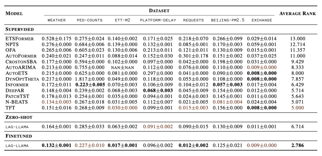
Table 1 presents the comparative results of zero-shot performance and performance after fine-tuning on unseen datasets between the supervised baseline models trained on specific datasets. In the zero-shot setting, Lag-Llama’s performance is comparable to all baseline models, with an average ranking of 6.714. During fine-tuning, Lag-Llama achieved state-of-the-art performance on three datasets, with significant improvements across all other datasets. Notably, during fine-tuning, Lag-Llama achieved an average ranking of 2.786, outperforming the best supervised model by 2 points, indicating that if one were to choose a method without prior data knowledge, Lag-Llama would be the optimal choice. This clearly establishes Lag-Llama as a powerful foundation model that can be used on downstream datasets with various unknown data distributions without prior knowledge, which is a key feature that a foundation model should possess.

We now delve deeper into Lag-Llama’s performance. In zero-shot evaluations, Lag-Llama exhibits strong performance, particularly on platform latency and weather datasets, closely matching baseline models. Through fine-tuning, Lag-Llama shows continuous improvement in performance, significantly enhancing the quality of predictions compared to zero-shot inference. On three datasets, ETT-M2, weather, and requests, the fine-tuned version of Lag-Llama has significantly lower errors than all baseline models, becoming the state-of-the-art model. On a currency exchange dataset from an entirely new domain, showcasing new unseen frequencies, Lag-Llama demonstrates comparable zero-shot performance and achieves performance similar to state-of-the-art models during fine-tuning. This indicates that Lag-Llama performs well across different frequencies and domains, regardless of whether the model has encountered similar data during pre-training. Compared to the Informer, AutoFormer, and ETSFormer models, Lag-Llama achieved better average rankings in both zero-shot and fine-tuning settings, despite these models using complex inductive biases to model time series, while Lag-Llama employs a simple architecture, lags, covariates, and large-scale pre-training. Our observations suggest that in large-scale scenarios, transformer models with only decoders outperform other transformer architectures when used similarly to Lag-Llama. We note that similar results have been proven in the natural language processing domain (Tay et al., 2022), which studied the impact of inductive bias in large-scale settings; however, we emphasize that we are the first to point out that such results apply to time series, potentially opening doors for further research on the impact of inductive bias in time series in large-scale scenarios. Furthermore, compared to the OneFitsAll model (Zhou et al., 2023b), which fine-tuned the pre-trained Lag-Llama model for predictions, Lag-Llama achieved significantly better performance on all datasets except the Beijing-PM2.5 dataset, with a much better average ranking than that model. These results indicate that there is greater potential in fine-tuning the pre-trained Lag-Llama model on large-scale and diverse time series datasets compared to training a time series foundation model from scratch. A detailed study on the advantages and disadvantages of fine-tuning the Lag-Llama model versus training a time series foundation model from scratch will be a direction for future work.

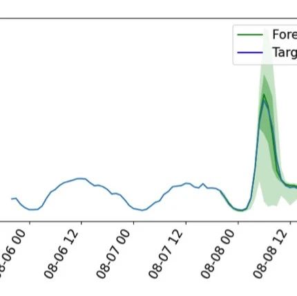
We also qualitatively illustrate the prediction results generated by Lag-Llama on unseen datasets in Appendix §E. The predictions generated by Lag-Llama are very close to the actual values. Moreover, comparing the predictions generated by the model in the zero-shot setting (Figure 8) and the predictions in the fine-tuning setting (Figure 11), it is clear that the quality of predictions significantly improves during fine-tuning.

Few-Shot Adaptation Performance on Unseen Data

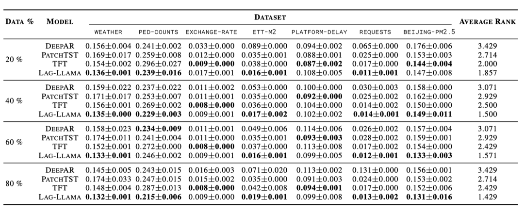
We limited the data to only use the last K% of historical data in the training set, where K is set to 20, 40, 60, and 80 percent, respectively. We trained supervised methods from scratch while fine-tuning Lag-Llama. The results are shown in Table 2. Across various degrees of available historical data, Lag-Llama achieved the best average ranking at all levels, indicating that Lag-Llama possesses strong adaptability across different data levels. As the amount of available historical data increases, Lag-Llama’s performance improves across all datasets, and the ranking gap between Lag-Llama and baseline models also widens, which is expected. However, it is noteworthy that on the currency exchange dataset from an entirely new domain with new unseen frequencies, Lag-Llama is often surpassed by TFT, indicating that when the data is least similar to the pre-training corpus, Lag-Llama requires more historical data for training, and under sufficient historical data for adaptation, its performance is comparable to state-of-the-art models (as discussed in Section 6.1).

Overall, our empirical results demonstrate that Lag-Llama possesses strong few-shot adaptation capabilities, and depending on the characteristics of the downstream datasets, Lag-Llama can adapt and generalize with an appropriate amount of data.

Analysis

Data Diversity

Although it has been found that loss is proportional to the size of the pre-training dataset (Kaplan et al., 2020), how other attributes of the pre-training dataset lead to ideal model behavior remains unclear, aside from some preliminary studies (Chan et al., 2022). Notably, the diversity of the pre-training data contributes to improved zero-shot performance and few-shot adaptability (Brown et al., 2020b), despite a lack of sufficient definition.

To quantify the diversity of the pre-training corpus, we analyze the characteristics of its datasets through 22 classic time series features (“catch22 features”), selected from features of the highly comparable time series analysis (hctsa) library, which are characterized by fast computation (Lubba et al., 2019). To assess the diversity of datasets, we average the features for each dataset and perform PCA analysis on the first two principal components. We find that having multiple datasets within-domain and across domains increases the diversity of AC22 features in the space of the first two principal components (see Figure 12 in the appendix).

Scale Analysis

It has been validated that the scale of datasets can improve performance (Kaplan et al., 2020). Constructing neural scaling laws (Kaplan et al., 2020; Caballero et al., 2023) can help us understand how model performance varies with different parameters (such as the amount of pre-training data, the number of parameters in the model, etc.). To understand these quantities for models like Lag-Llama, we fit the neural scaling laws to the validation loss of our model and present the scaling laws describing the relationship between our model’s performance and the amount of pre-training data in Appendix §F.1.

Discussion

We propose Lag-Llama, a univariate probabilistic time series forecasting foundation model based on a simple decoder-only transformer architecture. We demonstrate that Lag-Llama exhibits strong zero-shot generalization performance when pre-trained from scratch on large-scale datasets, comparable to models specific to certain datasets. After fine-tuning, Lag-Llama showcases state-of-the-art performance on diverse datasets from different domains and becomes the best general model without any downstream data knowledge. Lag-Llama also demonstrates strong few-shot adaptation performance at different levels of available data history. Finally, we explore the diversity of the pre-training corpus used to train Lag-Llama.

Our work opens several potential directions for future research. Currently, collecting and organizing large-scale open time series datasets would be of high value, as the largest time series dataset library (Godahewa et al., 2021) is too small by itself. Moreover, further expanding the model’s scale using different training strategies, beyond the model scale explored in this study, is an important next step in building more powerful time series foundation models. Lastly, extending our work from univariate to multivariate methods, capturing the complex multivariate dynamics of real-world datasets, is also a significant direction for future work.

Impact Statement

The goal of this research is to introduce a general foundation model for time series forecasting. Such models may have many social impacts, including positive effects through optimized processes via better decision-making, as well as potential negative impacts.

To our knowledge, the datasets used do not contain any personal or identifiable information, nor are they associated with it, and these datasets were obtained from cited sources.

Dataset Details

1. Table 3 further illustrates the presence of datasets in our pre-training or downstream testing corpus.

The Air Quality UC Irvine Repository dataset (UCI) contains 9,358 instances of hourly average responses from a chemical multi-sensor device embedded with five metal oxide chemical sensors in polluted areas (Vito, 2016).

The Australian Electricity Demand dataset includes half-hourly electricity demand time series from five states in Australia (Victoria, New South Wales, Queensland, Tasmania, and South Australia) (Godahewa et al., 2021).

The Beijing PM2.5 dataset contains hourly PM2.5 level data recorded by the US Embassy in Beijing. This dataset also includes meteorological data from Beijing Capital International Airport (Chen, 2017).

The Beijing Multi-Site Air-Quality dataset includes hourly measurement data of six major air pollutants and six corresponding meteorological variables across various locations in Beijing over four years (Chen, 2019).

The Electricity Hourly dataset records hourly electricity consumption for 321 customers during the period from 2012 to 2014 (Godahewa et al., 2021).

The ETTh1, ETTh2, ETTm1, ETTm2 datasets contain 2 years of data from two power transformers, obtained at hourly and 15-minute frequencies, for predicting whether the oil temperature of the power transformers is safe (Zhou et al., 2021b).

The Exchange Rate dataset includes daily exchange rates of eight foreign currencies from 1990 to 2016, namely Australia, the UK, Canada, Switzerland, China, Japan, New Zealand, and Singapore (Godahewa et al., 2021).

The Huawei cloud dataset contains serverless tracking data (Joosen et al., 2023). We selected eight series based on the median occurrence of the top 10 functions over a 141-day period at minute frequency: function latency, platform latency, CPU usage, memory usage, CPU limits, memory limits, instances, platform latency, and requests.

The London Smart Meters dataset focuses on the power consumption readings of 5,567 households participating in the UK Power Networks Low Carbon London project from November 2011 to February 2014 (Godahewa et al., 2021).

The KDD Cup 2018 dataset includes extensive hourly air quality level time series data from 59 sites in Beijing and London from January 2017 to March 2018. Measurements include PM2.5, PM10, NO2, CO, O3, and SO2 (Godahewa et al., 2021).

The Pedestrian Counts dataset (referred to as ped-counts in some parts of the text) includes hourly pedestrian counts recorded by 66 sensors within the city of Melbourne, starting from May 2009 (Godahewa et al., 2021).

The Solar dataset includes 5-minute solar power and hourly forecasts from 6,000 simulated solar power plants in the US in 2006. It includes 137 time series reflecting solar power generation every 10 minutes in Alabama in 2006 (Godahewa et al., 2021).

The Sunspot dataset includes an extensive daily sunspot number time series from January 1818 to May 2020 (Godahewa et al., 2021).

The Traffic dataset includes 862 hourly road occupancy time series in the San Francisco Bay Area from 2015 to 2016 (Godahewa et al., 2021).

The Uber TLC Hourly dataset includes 4.5 million Uber pickups in New York City (April to September 2014) and 14.3 million pickups (January to June 2015). It includes trip details from 10 other taxi companies and aggregated data from 329 companies (FiveThirtyEight; Godahewa et al., 2021).

The Weather dataset includes hourly climate data time series near Clayton Monash University in Victoria, Australia, spanning from January 2010 to May 2021. The data includes series of temperature, dew point temperature, wind speed, mean sea level pressure, relative humidity, surface solar radiation, surface thermal radiation, and total cloud cover (Godahewa et al., 2021).

The Wind Farms dataset includes minute frequency time series data tracking wind power generation from 339 wind farms in Australia (Godahewa et al., 2021).

Protocol Details

For all datasets used in the paper, we partitioned non-overlapping training and testing sets based on timestamps, as defined in the datasets. During pre-training, for each dataset, we excluded the last 14 overlapping windows in the training set and used them as the validation set for that dataset. During pre-training, we trained on the training set of each dataset, obtaining validation loss on the validation set of all datasets used in the pre-training corpus at the end of each epoch. We used the average validation loss as the early stopping criterion (referred to as “validation loss” in the paper). When fine-tuning on specific datasets, we excluded the last window in the training set and used it as the validation set for that dataset. We trained on the training set of the dataset and used the validation set for early stopping. We used the same settings for all supervised baseline models providing results in the paper as those used for fine-tuning Lag-Llama. According to typical evaluation settings (Shchur et al., 2023), all results reported in the paper are based on the results from the last prediction window of the testing set defined in App. §A.

Table 3: Datasets used in the pre-training corpus and the unseen datasets we evaluated, grouped by their respective domains.

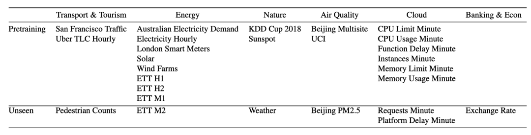
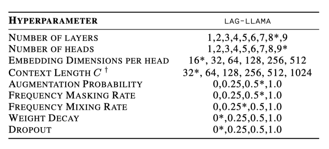
Table 5: Hyperparameter selection for Lag-Llama. Values with * indicate the best values obtained through hyperparameter search.

Note that this is just the context for continuously sampling for each window; in practice, due to the use of lags, we used a larger context window, as described in Section 4.1.

We plotted some sample prediction results and highlighted the median, the 50th (dark green), and the 90th (light green) prediction intervals; starting from datasets in the pre-training corpus: Figure 3 for Electricity Hourly, Figure 4 for ETT-H2, Figure 5 for Traffic. The zero-shot prediction results generated by Lag-Llama on downstream unseen datasets are highlighted in Figure 6 for ETT-M2, Figure 7 for Pedestrian Counts, and Figure 8 for Requests Minute. Finally, the prediction results after fine-tuning on these downstream unseen datasets are presented in Figure 9 for ETT-M2, Figure 10 for Pedestrian Counts, and Figure 11 for Requests Minute. Please pay special attention to the different magnitudes of sampled values based on the different datasets, through the same shared model.

Additional Empirical Results

Results on Pre-Training Datasets

A robust foundation model should excel in adapting to unseen data distributions in zero-shot and few-shot scenarios, but it should also perform well on the datasets used for model pre-training, i.e., exhibiting good internal performance on datasets. Therefore, in addition to evaluating our model on unseen datasets, we also assess our model on the datasets used for pre-training.

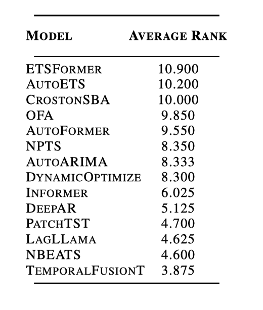
Results are shown in Tables 6, 7, and 8. The average ranking results for all datasets are shown in Table 9. Lag-Llama’s training budget is allocated to all pre-training datasets, while other supervised models do not have this restriction on datasets. Thus, the amount of data seen by Lag-Llama in each dataset is less than that of other models.

Hyperparameters of Lag-Llama

We randomly searched 100 different hyperparameter configurations and selected our model based on the average validation loss across all datasets in the pre-training corpus.

We list the possible hyperparameters for Lag-Llama and the best values obtained through our hyperparameter search in Table 5. Our final model was obtained through hyperparameter search, containing 2,449,299 parameters.

Prediction Visualization

We plotted some sample prediction results and highlighted the median, the 50th (deep green), and the 90th (light green) prediction intervals; starting from datasets in the pre-training corpus: Figure 3 for Electricity Hourly, Figure 4 for ETT-H2, Figure 5 for Traffic. The zero-shot prediction results generated by Lag-Llama on downstream unseen datasets are highlighted in Figure 6 for ETT-M2, Figure 7 for Pedestrian Counts, and Figure 8 for Requests Minute. Finally, the prediction results after fine-tuning on these downstream unseen datasets are presented in Figure 9 for ETT-M2, Figure 10 for Pedestrian Counts, and Figure 11 for Requests Minute. Please pay special attention to the different magnitudes of sampled values based on the different datasets, through the same shared model.

Additional Visualizations

Neural Scaling Laws

The parameter fitting of neural scaling laws (Caballero et al., 2023) is shown in Figure 13, fitting the validation loss with respect to the training periods of pre-training data (where each period consists of 100 randomly sampled windows). The specific parameters are as follows:

With such a law, we can infer the validation loss of the model and predict performance across a broader range of datasets (Figure 13). As efforts are made to compile better databases for training time series foundation models, these laws can help quantify the relationship between the data used and model performance.

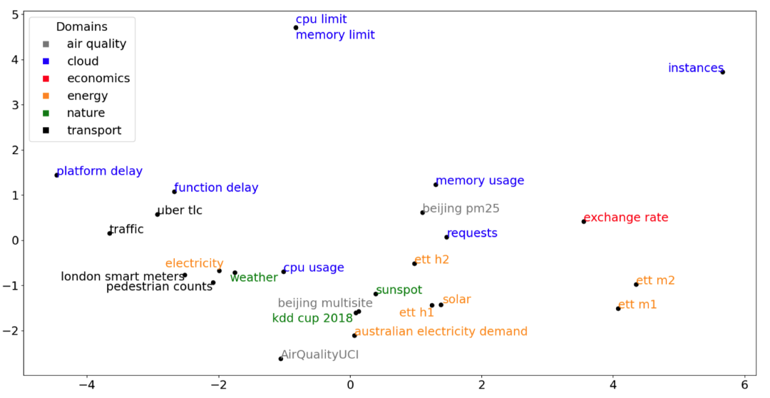
Table 9: Average rankings of all pre-training datasets. Lower values are better.