Click the above “Beginner Learning Vision”, select “Star” or “Top”
Heavyweight content delivered first-hand
What is OpenCV?
What Will I Learn?
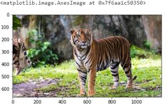
Reading and Displaying Images
import numpy as np
import cv2 as cv
import matplotlib.pyplot as plt
img=cv2.imread('../input/images-for-computer-vision/tiger1.jpg')print(type(img))
print(img.shape)# Converting image from BGR to RGB for displaying
img_convert=cv.cvtColor(img, cv.COLOR_BGR2RGB)
plt.imshow(img_convert)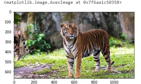
Drawing on Images
# Rectangle
color=(240,150,240) # Color of the rectangle
cv.rectangle(img, (100,100),(300,300),color,thickness=10, lineType=8) ## For filled rectangle, use thickness = -1
## (100,100) are (x,y) coordinates for the top left point of the rectangle and (300, 300) are (x,y) coordinates for the bottom right point
# Circle
color=(150,260,50)
cv.circle(img, (650,350),100, color,thickness=10) ## For filled circle, use thickness = -1
## (250, 250) are (x,y) coordinates for the center of the circle and 100 is the radius# Text
color=(50,200,100)
font=cv.FONT_HERSHEY_SCRIPT_COMPLEX
cv.putText(img, 'Save Tigers',(200,150), font, 5, color,thickness=5, lineType=20)# Converting BGR to RGB
img_convert=cv.cvtColor(img, cv.COLOR_BGR2RGB)
plt.imshow(img_convert)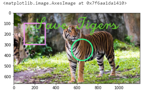
Merging Images
# For plotting multiple images at once
def myplot(images,titles):
    fig, axs=plt.subplots(1,len(images),sharey=True)
    fig.set_figwidth(15)
    for img,ax,title in zip(images,axs,titles):
        if img.shape[-1]==3:
            img=cv.cvtColor(img, cv.COLOR_BGR2RGB) # OpenCV reads images as BGR, so converting back them to RGB
        else:
            img=cv.cvtColor(img, cv.COLOR_GRAY2BGR)
        ax.imshow(img)
        ax.set_title(title)
img1 = cv.imread('../input/images-for-computer-vision/tiger1.jpg')
img2 = cv.imread('../input/images-for-computer-vision/horse.jpg')# Resizing the img1
img1_resize = cv.resize(img1, (img2.shape[1], img2.shape[0]))# Adding, Subtracting, Multiplying and Dividing Images
img_add = cv.add(img1_resize, img2)
img_subtract = cv.subtract(img1_resize, img2)
img_multiply = cv.multiply(img1_resize, img2)
img_divide = cv.divide(img1_resize, img2)# Blending Images
img_blend = cv.addWeighted(img1_resize, 0.3, img2, 0.7, 0) ## 30% tiger and 70% horse
myplot([img1_resize, img2], ['Tiger','Horse'])
myplot([img_add, img_subtract, img_multiply, img_divide, img_blend], ['Addition', 'Subtraction', 'Multiplication', 'Division', 'Blending'])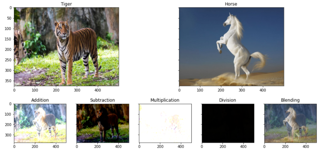
Image Transformations
img=cv.imread('../input/images-for-computer-vision/tiger1.jpg')

width, height, _=img.shape


# Translating
M_translate=np.float32([[1,0,200],[0,1,100]]) # 200=> Translation along x-axis and 100=>translation along y-axis

img_translate=cv.warpAffine(img,M_translate,(height,width))


# Rotating
center=(width/2,height/2)

M_rotate=cv.getRotationMatrix2D(center, angle=90, scale=1)

img_rotate=cv.warpAffine(img,M_rotate,(width,height))


# Scaling
scale_percent = 50

width = int(img.shape[1] * scale_percent / 100)

height = int(img.shape[0] * scale_percent / 100)

dim = (width, height)

img_scale = cv.resize(img, dim, interpolation = cv.INTER_AREA)


# Flipping
img_flip=cv.flip(img,1) # 0:Along horizontal axis, 1:Along vertical axis, -1: first along vertical then horizontal


# Shearing
srcTri = np.array( [[0, 0], [img.shape[1] - 1, 0], [0, img.shape[0] - 1]] ).astype(np.float32)
dstTri = np.array( [[0, img.shape[1]*0.33], [img.shape[1]*0.85, img.shape[0]*0.25], [img.shape[1]*0.15, img.shape[0]*0.7]] ).astype(np.float32)
warp_mat = cv.getAffineTransform(srcTri, dstTri)

img_warp = cv.warpAffine(img, warp_mat, (height, width))


myplot([img, img_translate, img_rotate, img_scale, img_flip, img_warp],
       ['Original Image', 'Translated Image', 'Rotated Image', 'Scaled Image', 'Flipped Image', 'Sheared Image'])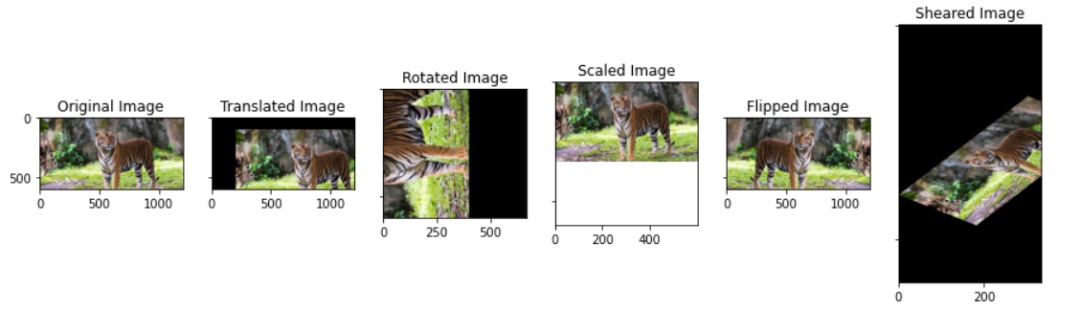
Image Preprocessing
# For visualising the filters
import plotly.graph_objects as go
from plotly.subplots import make_subplots
def plot_3d(img1, img2, titles):
    fig = make_subplots(rows=1, cols=2,
                    specs=[[{'is_3d': True}, {'is_3d': True}]],
                    subplot_titles=[titles[0], titles[1]],
                    )
    x, y=np.mgrid[0:img1.shape[0], 0:img1.shape[1]]
    fig.add_trace(go.Surface(x=x, y=y, z=img1[:,:,0]), row=1, col=1)
    fig.add_trace(go.Surface(x=x, y=y, z=img2[:,:,0]), row=1, col=2)
    fig.update_traces(contours_z=dict(show=True, usecolormap=True,
                                  highlightcolor="limegreen", project_z=True))
    fig.show()
img=cv.imread('../input/images-for-computer-vision/simple_shapes.png')
# Pixel value less than threshold becomes 0 and more than threshold becomes 255
_,img_threshold=cv.threshold(img,150,255,cv.THRESH_BINARY)
plot_3d(img, img_threshold, ['Original Image', 'Threshold Image=150'])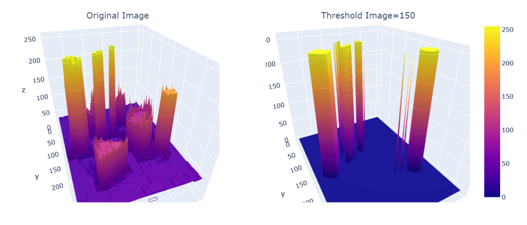
img=cv.imread('../input/images-for-computer-vision/simple_shapes.png')# Gaussian Filter
ksize=(11,11) # Both should be odd numbers
img_guassian=cv.GaussianBlur(img, ksize,0)
plot_3d(img, img_guassian, ['Original Image','Guassian Image'])# Median Filter
ksize=11
img_medianblur=cv.medianBlur(img,ksize)
plot_3d(img, img_medianblur, ['Original Image','Median blur'])# Bilateral Filter
img_bilateralblur=cv.bilateralFilter(img,d=5, sigmaColor=50, sigmaSpace=5)
myplot([img, img_bilateralblur],['Original Image', 'Bilateral blur Image'])
plot_3d(img, img_bilateralblur, ['Original Image','Bilateral blur'])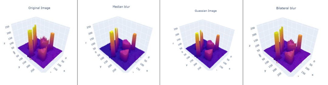
Feature Detection
Edge Detection
img=cv.imread('../input/images-for-computer-vision/simple_shapes.png')
img_canny1=cv.Canny(img,50, 200)
# Smoothing the img before feeding it to canny
filter_img=cv.GaussianBlur(img, (7,7), 0)
img_canny2=cv.Canny(filter_img,50, 200)
myplot([img, img_canny1, img_canny2],
       ['Original Image', 'Canny Edge Detector(Without Smoothing)', 'Canny Edge Detector(With Smoothing)'])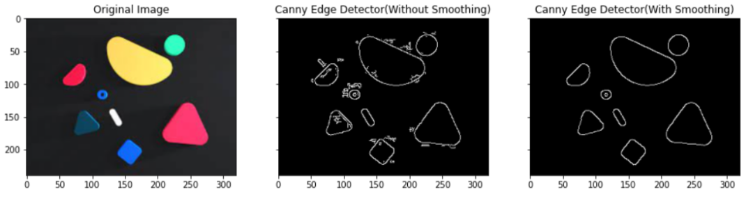
Contours
img=cv.imread('../input/images-for-computer-vision/simple_shapes.png')
img_copy=img.copy()
img_gray=cv.cvtColor(img,cv.COLOR_BGR2GRAY)
_,img_binary=cv.threshold(img_gray,50,200,cv.THRESH_BINARY)
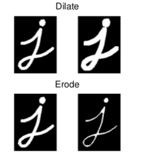
# Edroing and Dilating for smooth contours
img_binary_erode=cv.erode(img_binary,(10,10), iterations=5)
img_binary_dilate=cv.dilate(img_binary,(10,10), iterations=5)
contours,hierarchy=cv.findContours(img_binary,cv.RETR_TREE, cv.CHAIN_APPROX_SIMPLE)
cv.drawContours(img, contours,-1,(0,0,255),3) # Draws the contours on the original image just like draw function
myplot([img_copy, img], ['Original Image', 'Contours in the Image'])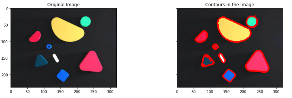
Hulls
img=cv.imread('../input/images-for-computer-vision/simple_shapes.png',0)
_,threshold=cv.threshold(img,50,255,cv.THRESH_BINARY)
contours,hierarchy=cv.findContours(threshold,cv.RETR_TREE, cv.CHAIN_APPROX_SIMPLE)
hulls=[cv.convexHull(c) for c in contours]
img_hull=cv.drawContours(img, hulls,-1,(0,0,255),2) # Draws the contours on the original image just like draw function
plt.imshow(img)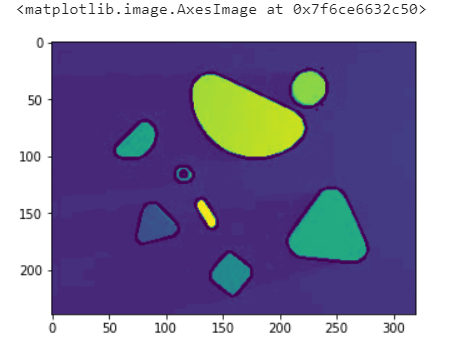
Conclusion
Good news!
The Beginner Learning Vision Knowledge Planet is now open to the public👇👇👇


Download 1: OpenCV-Contrib Extension Module Chinese Tutorial
Reply "Extension Module Chinese Tutorial" in the background of the "Beginner Learning Vision" public account to download the first OpenCV extension module tutorial in Chinese on the internet, covering installation of extension modules, SFM algorithms, stereo vision, target tracking, biological vision, super-resolution processing, and more than twenty chapters of content.

Download 2: 52 Lectures on Python Vision Practical Projects
Reply "Python Vision Practical Projects" in the background of the "Beginner Learning Vision" public account to download 31 visual practical projects including image segmentation, mask detection, lane line detection, vehicle counting, eyeliner addition, license plate recognition, character recognition, emotion detection, text content extraction, and face recognition, to help quickly learn computer vision.

Download 3: 20 Lectures on OpenCV Practical Projects
Reply "OpenCV Practical Projects 20 Lectures" in the background of the "Beginner Learning Vision" public account to download 20 practical projects based on OpenCV to advance learning of OpenCV.

Group Chat

Welcome to join the reader group of the public account to communicate with peers. There are currently WeChat groups for SLAM, 3D vision, sensors, autonomous driving, computational photography, detection, segmentation, recognition, medical imaging, GAN, algorithm competitions, etc. (will gradually be subdivided in the future). Please scan the WeChat number below to join the group, and note: "Nickname + School/Company + Research Direction", for example: "Zhang San + Shanghai Jiao Tong University + Visual SLAM". Please follow the format, otherwise, it will not be approved. After successful addition, you will be invited to join relevant WeChat groups based on research direction. Please do not send advertisements in the group, otherwise, you will be removed from the group. Thank you for understanding~