In-Depth Understanding of Attention Mechanism in CV

Hello everyone, I am Canshi.

In the field of deep learning, there are many technical terms that can be confusing when first encountered. As you read more, you gradually get the hang of it, but it still feels somewhat lacking. Today, we will discuss a technical term called Attention mechanism!

1. Intuitive Understanding of Attention

Imagine a scenario where you are driving (actually driving! The kind where you hold the steering wheel! Not the other kind of driving!), and it starts to rain, as shown in the figure below.

Now, if you want to see the road clearly, what do you need to do? That’s right! You smartly turn on the windshield wipers!

The action of the wiper clearing the rain can be thought of as the process of finding the Attention area! Yes! Give yourself a round of applause, you have understood the Attention mechanism!

2. Further Look at the Attention Mechanism

First, we introduce a concept called Key-Value, key-value pairs. The data types in this context are stored as key-value pairs, which is equivalent to a one-to-one concept (for example, in marriage law, a legal couple is a one-to-one relationship).

dict = {'name': 'canshi'}   # name is canshi

Recall back to high school, we learned about image formation in the eyes! An image in the eye is an inverted scaled image, and then the brain corrects it. We start modeling, assuming that the things that exist in nature are Key, also called Value.

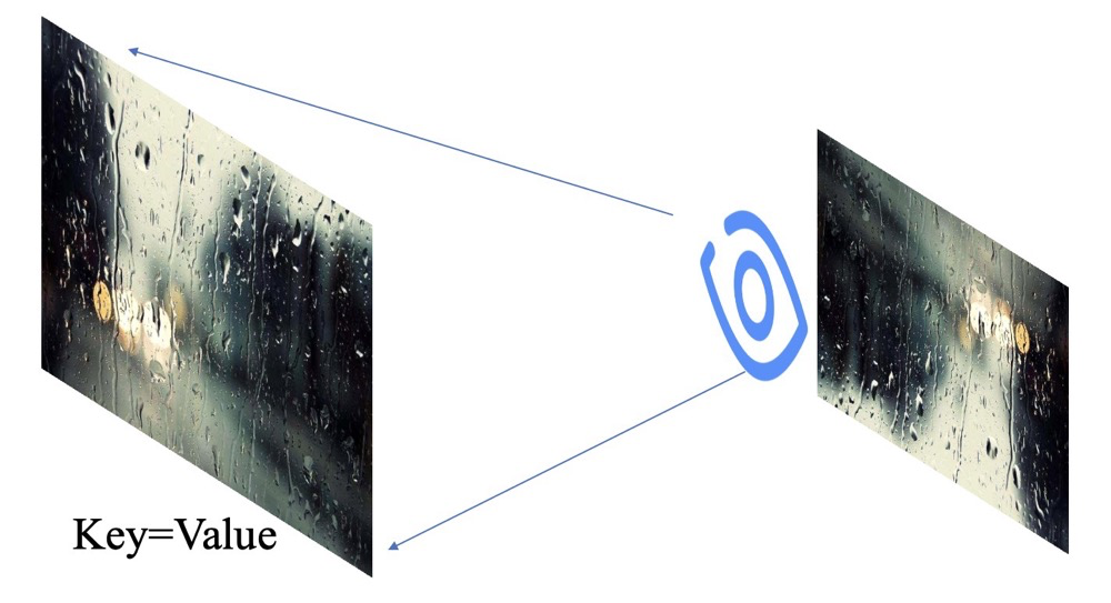
Using the formula, when it rains, the cold ice rain hits the car window hard! We call the entire window being hit Key, which is also called Value. But we can’t see the road clearly, so we want to distinguish the main information on the road, without needing the peripheral details. At this point, the wiper comes into play, which we call Query! We can then obtain a clearer image of the main road!

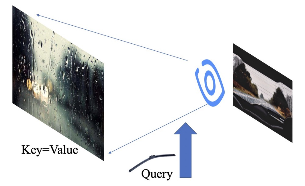
So what exactly happened? Let me break it down:

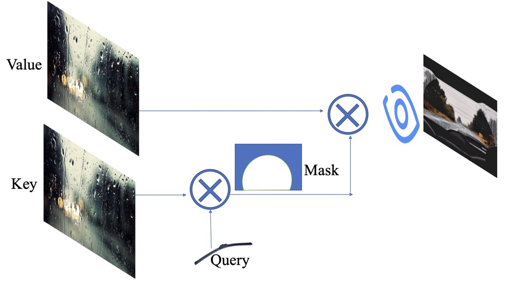
Thus, we use the wiper() to act on the window image(), obtaining a partially cleaned image (where the values inside are between 0 and 1), with the white areas in the image representing the cleaned parts, while the others are not relevant. We then multiply this generated Attention with the Value to get a partially cleaned generated image displayed in our brain.

Therefore, we often see the following diagrams in blogs discussing this:

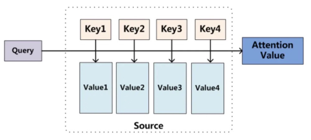
This diagram is mainly used in machine translation, where during translation, each output needs to calculate the similarity with each input element, and then perform a weighted sum.

In the field, we generally use matrix operations, unlike in tasks where time is a factor. In these tasks, it’s a matrix operation that can be completed in one go.

For example, during the process of the wiper clearing the rain, we denote the original window with rain as X, and the action of the wiper wiping the rain as W. We use similarity to replace the wiping process, obtaining an Attention. Then, we compute X with the generated Attention to get the final image.

Thus, the formula can be summarized as:

Highlighting the point, different cars have different wipers for clearing rain, similarly, we have different methods to measure similarity. Here we mainly have the following methods to measure similarity:

Once we have the similarity, we need to normalize it, organizing the original calculated scores into a probability distribution where the sum of all element weights equals 1, with more important parts being larger and less important parts being smaller. We primarily use the softmax function, although some use other methods for calculations, both are acceptable.

Therefore, the value of this weight can be calculated as:

Where it indicates scaling down the data to prevent it from becoming too large.

Finally, we get the output:

Thus, wearing glasses is also a way to focus on areas within the eyes, while other areas do not need any extra processing.

3. Attention Mechanism in the Brain

As people grow, every stage may involve training the brain to quickly obtain the information we want in nature. In the current big data era, with so many images and videos, we need to quickly browse to get information, as shown in the image below:

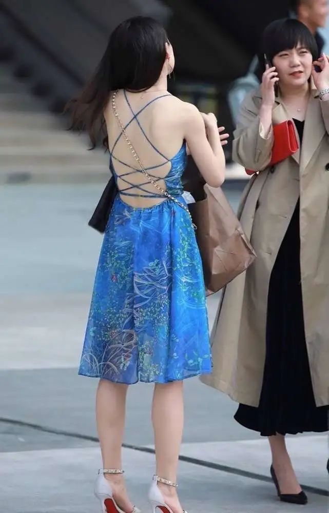
I might initially notice that the coat has a very good style, and that the red small bag is also nice. Of course, each person’s training dataset is different, and I don’t know what you all noticed first! After all, this attention matrix requires a massive amount of data for testing.

Oh? Still trying to argue with me? Then why don’t you try the challenge below?

The original video is from B station, not P station!

4. Common Attention Mechanisms in CV

1. Non-local Attention

From the above example, we understand that the essence is to calculate the weight matrix along one dimension. If this dimension is spatial, then it is Spatial Attention, if it is along the channel dimension, then it is Channel Attention. So, if you submit in the future and say you don’t have enough, we can just build a module out of it!

Here we use Self-Attention to explain the common Attention used in the field.

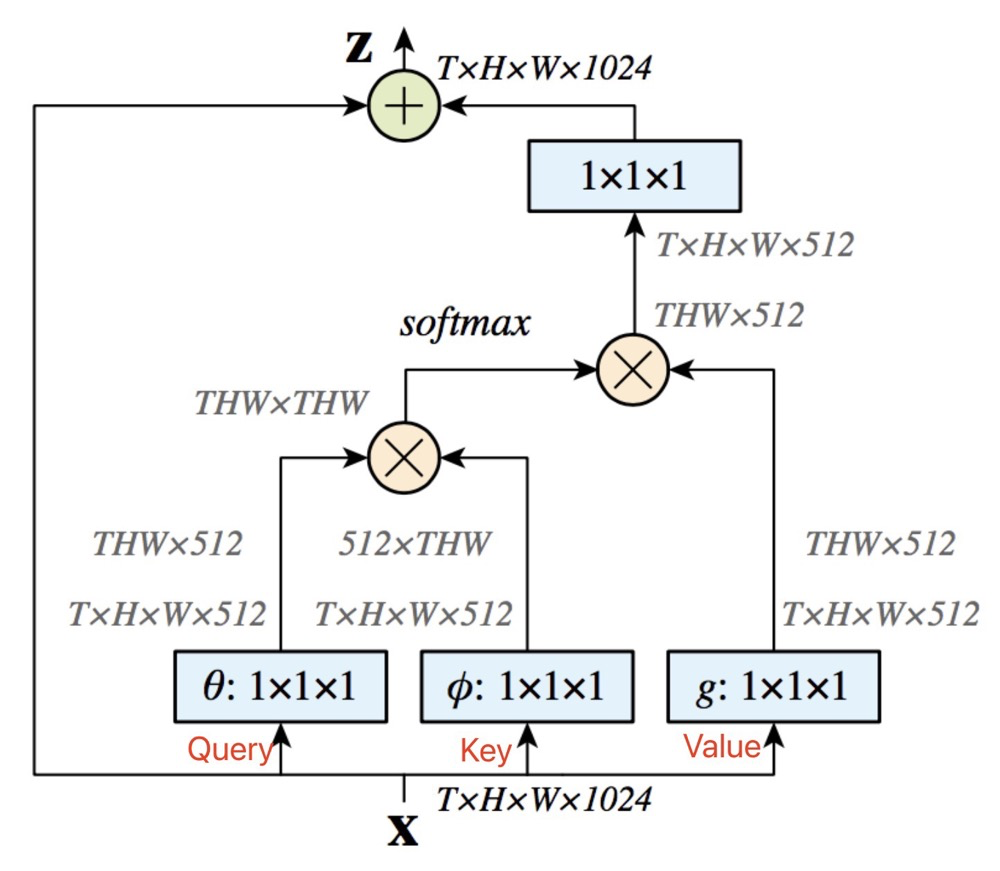
The input features are obtained through convolution, with three matrices being different, hence the previous assumption of similarity.

The code is as follows:

class Self_Attn(nn.Module):
    """ Self attention Layer"""
    def __init__(self,in_dim,activation):
        super(Self_Attn,self).__init__()
        self.chanel_in = in_dim
        self.activation = activation
        
        self.query_conv = nn.Conv2d(in_channels = in_dim , out_channels = in_dim//8 , kernel_size= 1)
        self.key_conv = nn.Conv2d(in_channels = in_dim , out_channels = in_dim//8 , kernel_size= 1)
        self.value_conv = nn.Conv2d(in_channels = in_dim , out_channels = in_dim , kernel_size= 1)
        self.gamma = nn.Parameter(torch.zeros(1))

        self.softmax  = nn.Softmax(dim=-1) #
    def forward(self,x):
        """
            inputs :
                x : input feature maps( B X C X W X H)
            returns :
                out : self attention value + input feature 
                attention: B X N X N (N is Width*Height)
        """
        m_batchsize,C,width ,height = x.size()
        proj_query  = self.query_conv(x).view(m_batchsize,-1,width*height).permute(0,2,1) # B X CX(N)
        proj_key =  self.key_conv(x).view(m_batchsize,-1,width*height) # B X C x (*W*H)
        energy =  torch.bmm(proj_query,proj_key) # transpose check
        attention = self.softmax(energy) # BX (N) X (N) 
        proj_value = self.value_conv(x).view(m_batchsize,-1,width*height) # B X C X N

        out = torch.bmm(proj_value,attention.permute(0,2,1) )
        out = out.view(m_batchsize,C,width,height)
        
        out = self.gamma*out + x
        return out,attention

The code appears to be relatively easy to understand; the main function allows for the multiplication of matrices with different dimensions to obtain the resultant matrix. Then it uses the softmax function to get the normalized matrix, combining with residuals to obtain the final output!

2. CBAM

It is composed of Channel Attention and Spatial Attention.

The Channel Attention module learns a weight matrix of size C x 1 x 1 from the dimension of C x H x W.

The diagram from the paper is as follows:

The code example is as follows:

class ChannelAttentionModule(nn.Module):
   def __init__(self, channel, reduction=16):
       super(ChannelAttentionModule, self).__init__()
       mid_channel = channel // reduction
       self.avg_pool = nn.AdaptiveAvgPool2d(1)
       self.max_pool = nn.AdaptiveMaxPool2d(1)

       self.shared_MLP = nn.Sequential(
           nn.Linear(in_features=channel, out_features=mid_channel),
           nn.ReLU(inplace=True),
           nn.Linear(in_features=mid_channel, out_features=channel)
       )
       self.sigmoid = nn.Sigmoid()

   def forward(self, x):
       avgout = self.shared_MLP(self.avg_pool(x).view(x.size(0),-1)).unsqueeze(2).unsqueeze(3)
       maxout = self.shared_MLP(self.max_pool(x).view(x.size(0),-1)).unsqueeze(2).unsqueeze(3)
       return self.sigmoid(avgout + maxout)

Of course, we can modify it into a unified architecture using MLP, as long as we can learn a distribution matrix across the channel dimension.

As shown in the pseudo-code below, all are generated by convolution.

# key: (N, C, H, W)
# query: (N, C, H, W)
# value: (N, C, H, W)
key = key_conv(x)
query = query_conv(x)
value = value_conv(x)

mask = nn.softmax(torch.bmm(key.view(N, C, H*W), query.view(N, C, H*W).permute(0,2,1)))
out = (mask * value.view(N, C, H*W)).view(N, C, H, W)

For Spatial Attention, as shown in the figure:

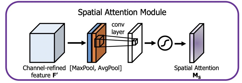
The reference code is as follows:

class SpatialAttentionModule(nn.Module):
    def __init__(self):
        super(SpatialAttentionModule, self).__init__()
        self.conv2d = nn.Conv2d(in_channels=2, out_channels=1, kernel_size=7, stride=1, padding=3)
        self.sigmoid = nn.Sigmoid()

    def forward(self, x):
        avgout = torch.mean(x, dim=1, keepdim=True)
        maxout, _ = torch.max(x, dim=1, keepdim=True)
        out = torch.cat([avgout, maxout], dim=1)
        out = self.sigmoid(self.conv2d(out))
        return out

Using MLP to rewrite:

key = key_conv(x)
query = query_conv(x)
value = value_conv(x)

b, c, h, w = t.size()
query = query.view(b, c, -1).permute(0, 2, 1)
key = key.view(b, c, -1)
value = value.view(b, c, -1).permute(0, 2, 1)

att = torch.bmm(query, key)

if self.use_scale:
  att = att.div(c**0.5)

att = self.softmax(att)
x = torch.bmm(att, value)

x = x.permute(0, 2, 1)
x = x.contiguous()
x = x.view(b, c, h, w)

3. CGNL

The paper analyzes that neither Channel Attention nor Spatial Attention can well describe the relationships between features, leading to the extreme generation of N * 1 * 1 * 1.

Key parts of the calculation code:

def kernel(self, t, p, g, b, c, h, w):
        """The linear kernel (dot production).
        Args:
            t: output of conv theta
            p: output of conv phi
            g: output of conv g
            b: batch size
            c: channels number
            h: height of featuremaps
            w: width of featuremaps
        """
        t = t.view(b, 1, c * h * w)
        p = p.view(b, 1, c * h * w)
        g = g.view(b, c * h * w, 1)

        att = torch.bmm(p, g)

        if self.use_scale:
            att = att.div((c*h*w)**0.5)

        x = torch.bmm(att, t)
        x = x.view(b, c, h, w)

        return x

4. Cross-layer Non-local

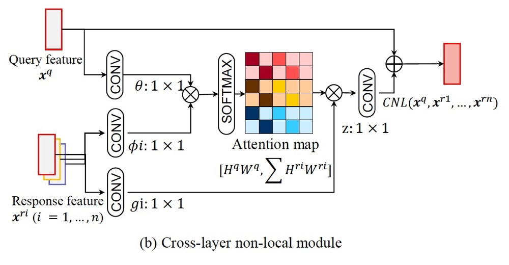
The paper analyzes that computing between the same layers can cause redundancy and introduce background noise, as shown in the left part of the figure. The right part shows that different layers have different receptive fields, and global computation will focus on more reasonable areas.

Here we adopt generation between layers.

The code part is quite interesting:

# query : N, C1, H1, W1
# key: N, C2, H2, W2
# value: N, C2, H2, W2
# First, we need to use 1 x 1 convolution to make the number of channels equal
q = query_conv(query) # N, C, H1, W1
k = key_conv(key) # N, C, H2, W2
v = value_conv(value) # N, C, H2, W2
att = nn.softmax(torch.bmm(q.view(N, C, H1*W1).permute(0, 1, 2), k.view(N, C, H2 * W2))) # (N, H1*W1, H2*W2)
out = att * value.view(N, C2, H2*W2).permute(0, 1, 2) #(N, H1 * W1, C)
out = out.view(N, C1, H1, W1)

4. Summary

This is a relatively suitable knowledge point for writing articles, considered a highlight. Currently, this can be summarized for the field, and I will continue to supplement it later. Everyone is welcome to follow!

– END –