
KNN Practical Application – Improving Matchmaking Effectiveness

Introduction
In simple terms, the KNN algorithm classifies data by measuring the distances between different feature values. The working principle is that there exists a sample dataset, namely the training dataset, and each sample in the dataset has a label, which indicates the correspondence between each data point and its classification. When new unlabeled data is inputted, the algorithm compares each feature of the new data with the corresponding features in the sample dataset, then extracts the classification label of the most similar data (nearest neighbor) from the sample set. Generally, only the top K most similar data points from the sample dataset are selected, which is the origin of ‘k’ in the KNN algorithm, and K is usually an integer greater than 20. Finally, the classification that appears most frequently among the K most similar data points is taken as the classification for the new data.
Advantages: High accuracy, insensitive to outliers, no data input assumptions.
Disadvantages: High computational complexity, high space complexity.
Applicable scope: Numerical and nominal data.
Today we will use the KNN algorithm to improve the matchmaking effectiveness of a dating website. First, let’s introduce the background of this practical application.
Background Introduction
A beautiful girl named Er Ya is looking for a suitable dating partner on an online dating website. Although the website recommends different candidates, she does not like everyone. After some summarization, she found that she had previously dated three types of people:
People she does not like.
People with average charm.
People with great charm.
Despite discovering these patterns, Er Ya still cannot categorize the recommended matches from the dating website correctly. She can date those with average charm from Monday to Friday and those with great charm on weekends. Therefore, she hopes we can help her design a system that categorizes different candidates appropriately. For this purpose, Er Ya has also provided some necessary information.
Algorithm Flow
Collect data: Provide a text file.
Prepare data: Use Python to parse the text file.
Analyze data: Use Matplotlib to create a 2D plot.
Train data:
Test algorithm: Use part of the data provided by Er Ya as the test set.
Deploy algorithm: Generate a simple command-line program, allowing Er Ya to input some feature data to determine if the other person is her preferred type.
1. Prepare Data: Parse Data from Text File
The data is stored in datingTestSet.txt, with each sample occupying one line, totaling 1000 lines. The samples mainly contain the following three features:
Annual flight mileage.
Percentage of time spent playing games.
Weekly consumption of ice cream in kilograms.
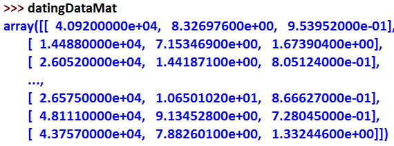
Convert text records into a Numpy parsing program:
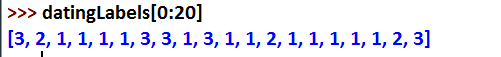
def file2matrix(filename): fr = open(filename) numberOfLines = len(fr.readlines()) #get the number of lines in the file returnMat = zeros((numberOfLines,3)) #prepare matrix to return classLabelVector = [] #prepare labels return fr = open(filename) index = 0 for line in fr.readlines(): line = line.strip() listFromLine = line.split(‘\t’) returnMat[index,:] = listFromLine[0:3] classLabelVector.append(int(listFromLine[-1])) index += 1 return returnMat,classLabelVector
This function is stored as a subfunction of the KNN function in kNN.py file. In the Python command line, input the following command:
>>> import sys>>> sys.path.append(‘C:\Users\NEU\Desktop\JKXY\machinelearninginaction\Ch02′)>>> import os>>> os.getcwd()’C:\Python26\Lib\idlelib’>>> os.chdir(‘C:\Users\NEU\Desktop\JKXY\machinelearninginaction\Ch02′)>>> os.getcwd()’C:\Users\NEU\Desktop\JKXY\machinelearninginaction\Ch02’>>> import kNN>>> datingDataMat, datintLabels = kNN.file2matrix(“datingTestSet2.txt”)
We have now imported the text file into the runtime environment and converted it into the required format. Next, we need to understand the specific meaning of the data. Therefore, we will use Python tools to visualize the data content to identify some data patterns.
2. Analyze Data: Create Scatter Plot Using Matplotlib
First, use Matplotlib to create a scatter plot of the raw data. Input the following command in the Python command line:
>>> import matplotlib>>> import matplotlib.pyplot as plt>>> fig = plt.figure()>>> ax = fig.add_subplot(111)>>> ax.scatter(datingDataMat[:,1], datingDataMat[:,2])<matplotlib.collections.CircleCollection object at 0x03C8A190>>>> plt.show()
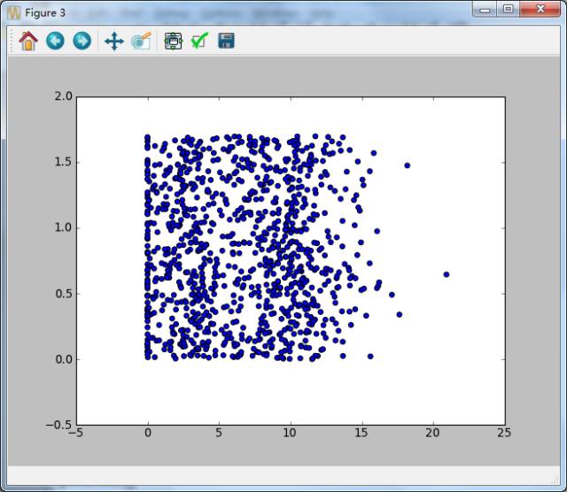
The scatter plot of dating data without category labels makes it difficult to identify which points belong to which category (“Percentage of time spent playing games” and “Weekly consumption of ice cream in kilograms”).
The second and third columns of datingDataMat represent the feature values of “Percentage of time spent playing games” and “Weekly consumption of ice cream in kilograms”, while the first column is the “Annual flight mileage”. Since we have not used the feature values of the sample classification, we cannot obtain any useful data pattern information from the above plot.
Re-enter the following command in the Python command line:
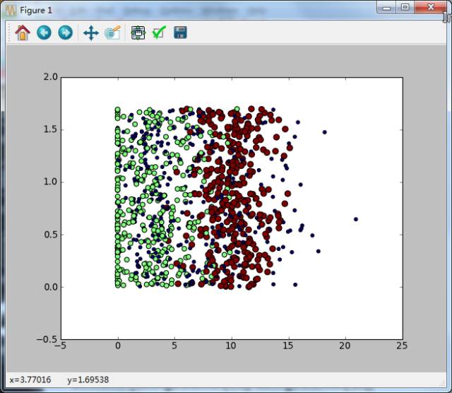
The scatter plot of dating data with category labels, although it is easier to distinguish which data points belong to which category, still makes it difficult to draw conclusive information from this chart (“Percentage of time spent playing games” and “Weekly consumption of ice cream in kilograms”).
The application of KNN to improve the matchmaking effectiveness of the dating website will be described in two articles. This blog post ends here. The next article will explain the normalization of the algorithm and the key parts of KNN (the Python implementation code will be provided in the next article).